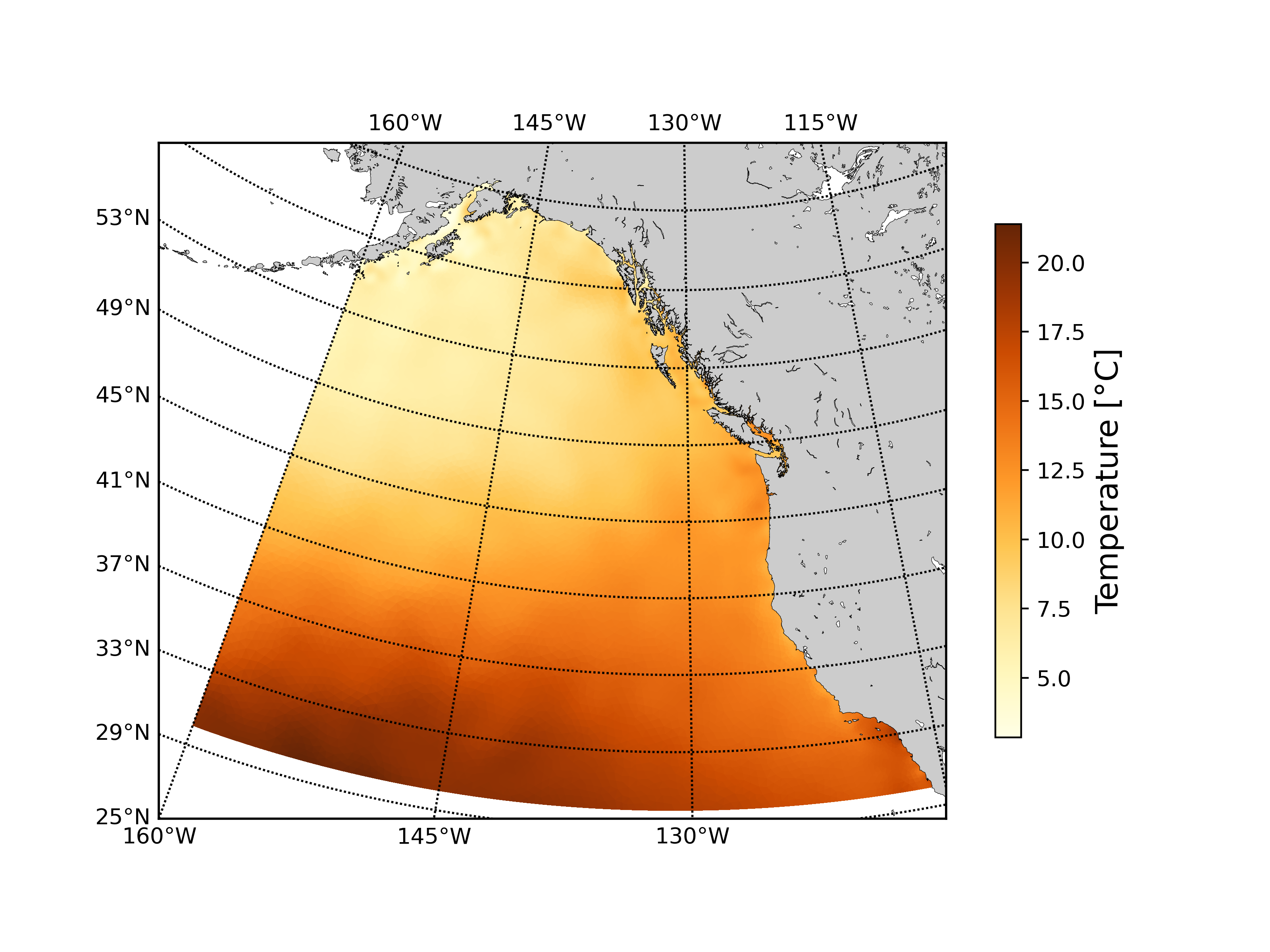
Description: Seasonal mean primary production from the British Columbia continental margin model (BCCM) were averaged over the 1981 to 2010 period and depth-integrated to create seasonal mean climatology of the Canadian Pacific Exclusive Economic Zone. Methods: Total primary production is the sum of diatoms and flagellates production. Spring months were defined as April to June, summer months were defined as July to September, fall months were defined as October to December, and winter months were defined as January to March. The data available here contain a raster layer of seasonal depth-integrated primary production climatology for the Canadian Pacific Exclusive Economic Zone at 3 km spatial resolution. Uncertainties: Model results have been extensively evaluated against observations (e.g. altimetry, CTD and nutrient profiles, observed geostrophic currents), which showed the model can reproduce with reasonable accuracy the main oceanographic features of the region including salient features of the seasonal cycle and the vertical and cross-shore gradient of water properties. However, the model resolution is too coarse to allow for an adequate representation of inlets, nearshore areas, and the Strait of Georgia.

Description: Seasonal mean temperature from the British Columbia continental margin model (BCCM) were averaged over the 1981 to 2010 period to create seasonal mean climatology of the Canadian Pacific Exclusive Economic Zone. Methods: Temperatures at up to forty-six linearly interpolated vertical levels from surface to 2400 m and at the sea bottom are included. Spring months were defined as April to June, summer months were defined as July to September, fall months were defined as October to December, and winter months were defined as January to March. The data available here contain raster layers of seasonal temperature climatology for the Canadian Pacific Exclusive Economic Zone at 3 km spatial resolution and 47 vertical levels. Uncertainties: Model results have been extensively evaluated against observations (e.g. altimetry, CTD and nutrient profiles, observed geostrophic currents), which showed the model can reproduce with reasonable accuracy the main oceanographic features of the region including salient features of the seasonal cycle and the vertical and cross-shore gradient of water properties. However, the model resolution is too coarse to allow for an adequate representation of inlets, nearshore areas, and the Strait of Georgia.

Description: Seasonal mean dissolved inorganic carbon concentration from the British Columbia continental margin model (BCCM) were averaged over the 1993 to 2020 period to create seasonal mean climatology of the Canadian Pacific Exclusive Economic Zone. Methods: Dissolved inorganic carbon concentrations at up to forty-six linearly interpolated vertical levels from surface to 2400 m and at the sea bottom are included. Spring months were defined as April to June, summer months were defined as July to September, fall months were defined as October to December, and winter months were defined as January to March. The data available here contain raster layers of seasonal dissolved inorganic carbon concentration climatology for the Canadian Pacific Exclusive Economic Zone at 3 km spatial resolution and 47 vertical levels. Uncertainties: Model results have been extensively evaluated against observations (e.g. altimetry, CTD and nutrient profiles, observed geostrophic currents), which showed the model can reproduce with reasonable accuracy the main oceanographic features of the region including salient features of the seasonal cycle and the vertical and cross-shore gradient of water properties. However, the model resolution is too coarse to allow for an adequate representation of inlets, nearshore areas, and the Strait of Georgia.

Description: Seasonal mean pH from the British Columbia continental margin model (BCCM) were averaged over the 1993 to 2020 period to create seasonal mean climatology of the Canadian Pacific Exclusive Economic Zone. Methods: The pH at up to forty-six linearly interpolated vertical levels from surface to 2400 m and at the sea bottom are included. Spring months were defined as April to June, summer months were defined as July to September, fall months were defined as October to December, and winter months were defined as January to March. The data available here contain raster layers of seasonal pH climatology for the Canadian Pacific Exclusive Economic Zone at 3 km spatial resolution and 47 vertical levels. Uncertainties: Model results have been extensively evaluated against observations (e.g. altimetry, CTD and nutrient profiles, observed geostrophic currents), which showed the model can reproduce with reasonable accuracy the main oceanographic features of the region including salient features of the seasonal cycle and the vertical and cross-shore gradient of water properties. However, the model resolution is too coarse to allow for an adequate representation of inlets, nearshore areas, and the Strait of Georgia.

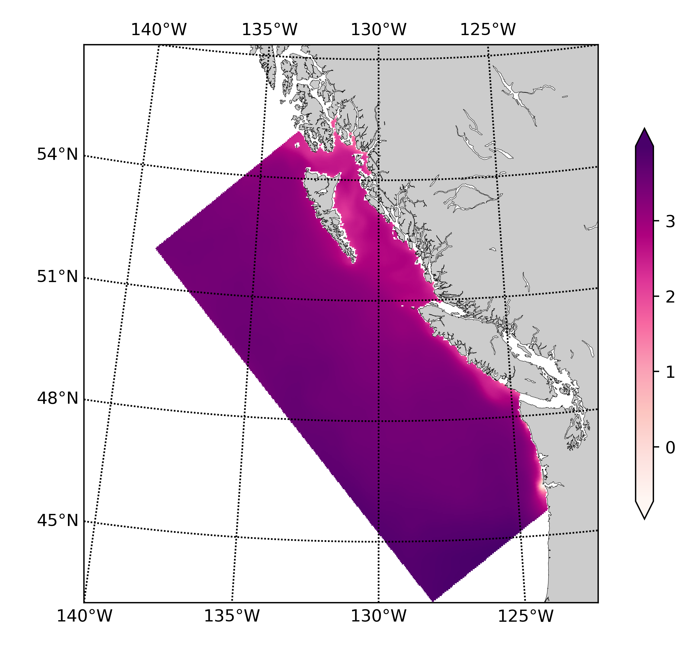
Description: Seasonal climatologies of the Canadian Pacific Exclusive Economic Zone (CPEEZ) were computed from a numerical simulation of the British Columbia continental margin (BCCM) model for the 1981 to 2010 period, which can be considered as a representation of the climatological state of the region. Methods: The BCCM model is an ocean circulation-biogeochemical model implementation of the Regional Ocean Modelling System (ROMS version 3.5). The horizontal resolution is eddy-resolving at 3 km and the vertical discretization is based on a terrain-following coordinate system with 42 depth levels of increasing resolution near the surface. A detailed description of the BCCM model is given in Peña et al. (2019). Spring months were defined as April to June, summer months were defined as July to September, fall months were defined as October to December, and winter months were defined as January to March. The data available here contain raster layers of seasonal climatology of temperature, salinity, current speed, nitrate, oxygen, total alkalinity, dissolved inorganic carbon, pH, aragonite saturation state, phytoplankton, and primary production. The data include 47 vertical levels (surface, bottom, and 45 more selected depths), except for total phytoplankton (surface values only) and primary production (depth-integrated values). A layer giving the bottom depth in metres at the centre of each grid point is also provided. Model grids were set to NaN values in regions where the model output is highly uncertain, such as inlets, nearshore areas, and the Strait of Georgia. Uncertainties: Model results have been compared against tide gauge data, altimetry, CTD and nutrient profiles, observed geostrophic currents, and seasonal temperature and salinity climatologies over the 1981 to 2010 period. The model is successful in reproducing the main features of the region including salient features of the seasonal cycle and the vertical structure of density and nutrients.

Description: This dataset consists of three simulations from the Northeastern Pacific Canadian Ocean Ecosystem Model (NEP36-CanOE) which is a configuration of the Nucleus for European Modelling of the Ocean (NEMO) V3.6. The historical simulation is an estimate of the 1986-2005 mean climate. The future simulations project the 2046-2065 mean climate for representative concentration pathways (RCP) 4.5 (moderate mitigation scenario) and 8.5 (no mitigation scenario). Each simulation is forced by a climatology of atmospheric forcing fields calculated over these 20 year periods and the winds are augmented with high frequency variability, which introduces a small amount of interannual variability. Model outputs are averaged over 3 successive years of simulation (the last 3, following an equilibration period); standard deviation among the 3 years is available upon request. For each simulation, the dataset includes the air-sea carbon dioxide flux, monthly 3D fields for potential temperature, salinity, potential density, total alkalinity, dissolved inorganic carbon, nitrate, oxygen, pH, total chlorophyll, aragonite saturation state, total primary production, and monthly maximum and minimum values for oxygen, pH, and potential temperature. The data includes 50 vertical levels at a 1/36 degree spatial resolution and a mask is provided that indicates regions where these data should be used cautiously or not at all. For a more detailed description please refer to Holdsworth et al. 2021. Methods: This study uses a multi-stage downscaling approach to dynamically downscale global climate projections at a 1/36° (1.5 − 2.25 km) resolution. We chose to use the second-generation Canadian Earth System model (CanESM2) because high-resolution downscaled projections of the atmosphere over the region of interest are available from the Canadian Regional Climate Model version 4 (CanRCM4). We used anomalies from CanESM2 with a resolution of about 1° at the open boundaries, and the regional atmospheric model, CanRCM4 (Scinocca et al., 2016) for the surface boundary conditions. CanRCM4 is an atmosphere only model with a 0.22° resolution and was used to downscale climate projections from CanESM2 over North America and its adjacent oceans. The model used is computationally expensive. This is due to the relatively high number of points in the domain (715 × 1,021 × 50) and the relatively complex biogeochemical model (19 tracers). Therefore, rather than carrying out interannual simulations for the historical and future periods, we implemented a new method that uses atmospheric climatologies with augmented winds to force the ocean. We show that augmenting the winds with hourly anomalies allows for a more realistic representation of the surface freshwater distribution than using the climatologies alone. Section 2.1 describes the ocean model that is used to estimate the historical climate and project the ocean state under future climate scenarios. The time periods are somewhat arbitrary; 1986–2005 was chosen because the Coupled Model Intercomparison Project Phase 5 (CMIP5) historical simulations end in 2005 as no community-accepted estimates of emissions were available beyond that date (Taylor et al., 2009); 2046–2065 was chosen to be far enough in the future that changes in 20 year mean fields are unambiguously due to changing GHG forcing (as opposed to model internal variability) (e.g., Christian, 2014), but near enough to be considered relevant for management purposes. While it is true that 30 years rather than 20 is the canonical value for averaging over natural variability, in practice the difference between a 20 and a 30 year mean is small (e.g., if we average successive periods of an unforced control run, the variance among 20 year means will be only slightly larger than for 30 year means). Also, there is concern that longer averaging periods are inappropriate in a non-stationary climate (Livezey et al., 2007; Arguez and Vose, 2011). We chose 20 year periods because they are adequate to give a mean annual cycle with little influence from natural variability, while minimizing aliasing of the secular trend into the means. As the midpoints of the two time periods are separated by 60 years, the contribution of natural variability to the differences between the historical and future simulations is negligible e.g., (Hawkins and Sutton, 2009; Frölicher et al., 2016). Section 2.2 describes how climatologies derived from observations were used for the initialization and open boundary conditions for the historical simulations and pseudo-climatologies were used for the future scenarios. The limited availability of observations means that the years used for these climatologies differs somewhat from the historical and future periods. Section 2.3 details the atmospheric forcing fields and the method that we developed to generate winds with realistic high-frequency variability while preserving the daily climatological means from the CanRCM4 data. Section 2.4 shows the equilibration of key modeled variables to the forcing conditions Data Sources: Model output Uncertainties: The historical climatologies were evaluated using observational climatologies generated from stations with a long time series of data over the time period including CTDs, nutrient profiles, lighthouse and satellite SST, and buoy data. The model is able to represent the historical conditions with an acceptable bias. The resolution of this model is insufficient to represent the narrow straits and channels of this region so the dataset includes a cautionary mask to exclude these regions.

Description: Seasonal mean salinity from the British Columbia continental margin model (BCCM) were averaged over the 1981 to 2010 period to create seasonal mean climatology of the Canadian Pacific Exclusive Economic Zone. Methods: Salinities at up to forty-six linearly interpolated vertical levels from surface to 2400 m and at the sea bottom are included. Spring months were defined as April to June, summer months were defined as July to September, fall months were defined as October to December, and winter months were defined as January to March. The data available here contain raster layers of seasonal salinity climatology for the Canadian Pacific Exclusive Economic Zone at 3 km spatial resolution and 47 vertical levels. Uncertainties: Model results have been extensively evaluated against observations (e.g. altimetry, CTD and nutrient profiles, observed geostrophic currents), which showed the model can reproduce with reasonable accuracy the main oceanographic features of the region including salient features of the seasonal cycle and the vertical and cross-shore gradient of water properties. However, the model resolution is too coarse to allow for an adequate representation of inlets, nearshore areas, and the Strait of Georgia.

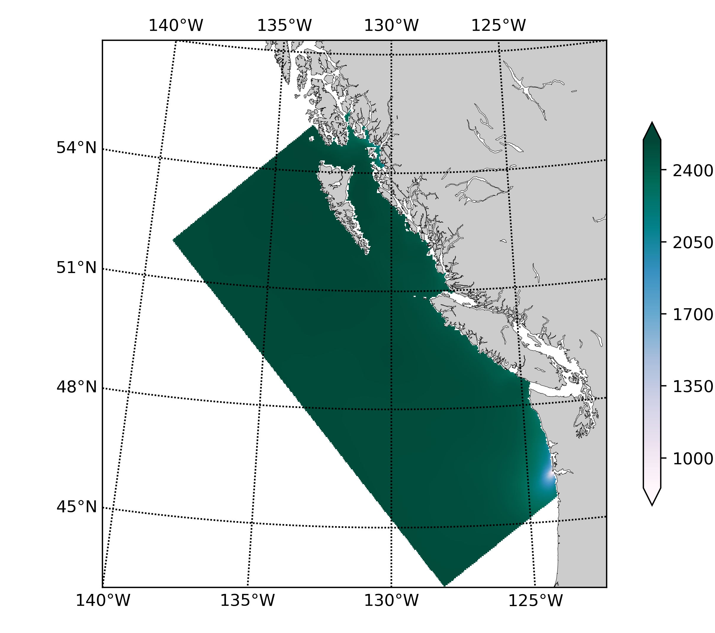
Description: Seasonal mean oxygen concentration from the British Columbia continental margin model (BCCM) were averaged over the 1993 to 2020 period to create seasonal mean climatology of the Canadian Pacific Exclusive Economic Zone. Methods: Oxygen concentrations at up to forty-six linearly interpolated vertical levels from surface to 2400 m and at the sea bottom are included. Spring months were defined as April to June, summer months were defined as July to September, fall months were defined as October to December, and winter months were defined as January to March. The data available here contain raster layers of seasonal oxygen concentration climatology for the Canadian Pacific Exclusive Economic Zone at 3 km spatial resolution and 47 vertical levels. Uncertainties: Model results have been extensively evaluated against observations (e.g. altimetry, CTD and nutrient profiles, observed geostrophic currents), which showed the model can reproduce with reasonable accuracy the main oceanographic features of the region including salient features of the seasonal cycle and the vertical and cross-shore gradient of water properties. However, the model resolution is too coarse to allow for an adequate representation of inlets, nearshore areas, and the Strait of Georgia.

Description: Seasonal mean current speed from the British Columbia continental margin model (BCCM) were calculated as the root mean square of the zonal (U) and meridional (V) velocities and averaged over the 1993 to 2020 period to create seasonal mean climatology of the Canadian Pacific Exclusive Economic Zone. Methods: Current speeds at up to forty-six linearly interpolated vertical levels from surface to 2400 m and at the sea bottom are included. Spring months were defined as April to June, summer months were defined as July to September, fall months were defined as October to December, and winter months were defined as January to March. The data available here contain raster layers of seasonal current speed climatology for the Canadian Pacific Exclusive Economic Zone at 3 km spatial resolution and 47 vertical levels. Uncertainties: Model results have been extensively evaluated against observations (e.g. altimetry, CTD and nutrient profiles, observed geostrophic currents), which showed the model can reproduce with reasonable accuracy the main oceanographic features of the region including salient features of the seasonal cycle and the vertical and cross-shore gradient of water properties. However, the model resolution is too coarse to allow for an adequate representation of inlets, nearshore areas, and the Strait of Georgia.

Description: Seasonal mean total alkalinity from the British Columbia continental margin model (BCCM) were averaged over the 1981 to 2010 period to create seasonal mean climatology of the Canadian Pacific Exclusive Economic Zone. Methods: Total alkalinities at up to forty-six linearly interpolated vertical levels from surface to 2400 m and at the sea bottom are included. Spring months were defined as April to June, summer months were defined as July to September, fall months were defined as October to December, and winter months were defined as January to March. The data available here contain raster layers of seasonal total alkalinity climatology for the Canadian Pacific Exclusive Economic Zone at 3 km spatial resolution and 47 vertical levels. Uncertainties: Model results have been extensively evaluated against observations (e.g. altimetry, CTD and nutrient profiles, observed geostrophic currents), which showed the model can reproduce with reasonable accuracy the main oceanographic features of the region including salient features of the seasonal cycle and the vertical and cross-shore gradient of water properties. However, the model resolution is too coarse to allow for an adequate representation of inlets, nearshore areas, and the Strait of Georgia.