The St. Lawrence Estuary is known as a summer foraging area for several species of marine mammals, including several species of rorquals. Among these is the blue whale, which feeds almost exclusively on euphausiids. Therefore, the abundance, distribution and local density of krill should logically be a strong explanatory variable for the distribution of blue whales. However little is known about the spatial association of blue whales with the aggregation dynamics of krill in eastern Canada. Six years of acoustic surveys, conducted in August from 2009 to 2014, were undertaken to study the medium- and small-scale distribution of krill within the northwestern Gulf of St. Lawrence and estuary. The data shows a mosaic of the maximum annual density of arctic krill (T. raschii) made from these surveys. McQuinn, I.H., Gosselin, J.-F., Bourassa, M.-N., Mosnier, A., St-Pierre, J.-F., Plourde, S., Lesage, V., Raymond, A. 2016. The spatial association of blue whales (Balaenoptera musculus) with krill patches (Thysanoessa spp. and Meganyctiphanes norvegica) in the estuary and northwestern Gulf of St. Lawrence. DFO Can. Sci. Advis. Sec. Res. Doc. 2016/104. iv + 19 p.

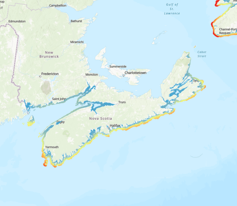
Exposure to wind-driven waves forms a key physical gradient in nearshore environments influencing both ecological communities and human activities. We calculated a relative exposure index (REI) for wind-driven waves covering the coastal zone of the Scotian Shelf-Bay of Fundy bioregion. We derived REI and two other fetch-based indices (sum fetch, minimum fetch) from two formulations of wind fetch (unweighted and effective fetch) for input points in an evenly spaced fishnet grid (50-m resolution) covering a buffered area within 5 km from the coastline and shallower than 50 m depth. We calculated unweighted fetch lengths (m) for 32 compass headings per input point (11.25° intervals), and effective fetch lengths for 8 headings per point (45° intervals). Unweighted fetch is the distance along a given heading from a point in coastal waters to land. Effective fetch is a directionally weighted average of multiple fetch measures around a given heading that reduces the influence of irregular coastline shape on exposure estimates. For fetch calculations, we used land features at a 1:50,000 scale for Canadian administrative boundaries (NrCan 2017), and unknown resolution for St. Pierre and Miquelon, and US states bordering the Gulf of Maine (GADM 2012). The summed and minimum unweighted fetch lengths for each point provide coarse summaries of wave exposure and distance to land, respectively. The relative exposure index (REI) gives a more accurate metric of exposure by combining effective fetch with modelled wind speeds (m s-1) and frequency data. We provide the original calculations of unweighted fetch, effective fetch, and other fetch-based indices (i.e., sum, minimum) in csv format along with the REI layer (GeoTIFF format) resampled to 35-m resolution. With broad spatial coverage and high resolution, these indices can support regional-scale distribution modelling of species and biological assemblages in the coastal zone as well as marine spatial planning activities. When using data please cite following: O'Brien JM, Wong MC, Stanley RRE (2022) A relative wave exposure index for the coastal zone of the Scotian Shelf-Bay of Fundy Bioregion. figshare. Collection. https://doi.org/10.6084/m9.figshare.c.5433567 References GADM database of Global Administrative Areas (2012). Global Administrative Areas, version 2.0. (accessed 2 December 2020). www.gadm.org Natural Resources Canada (2017) Administrative Boundaries in Canada - CanVec Series - Administrative Features - Open Government Portal. (accessed 2 December 2020). https://open.canada.ca/data/en/dataset/306e5004-534b-4110-9feb-58e3a5c3fd97.

“Prince Albert National Park - Total Ecosystem Forest Carbon Density” is the annual carbon density (tonnes carbon per hectare) within Prince Albert’s forested ecosystems over a 31-year period from 1990 to 2020. Total Ecosystem Forest Carbon Density includes aboveground and belowground biomass, soil carbon, and dead organic matter. Total Ecosystem Forest Carbon Density was estimated for 31 national parks using the Generic Carbon Budget Model (GCBM), a spatially explicit carbon budget model developed by Canadian Forest Service which uses forest inventory, disturbance, and mean annual temperature data along with yield data to estimate growth and merchantable volume for dominant tree species. Species- and Ecozone-specific equations are then used to convert merchantable volume to aboveground and belowground biomass carbon. Ecozones were classified according to Canada Ecological Land Classification Level 1. The GCBM simulates carbon dynamics to produce spatially explicit estimations of carbon stocks and fluxes. The model simulates and tracks carbon stocks, transfers between Intergovernmental Panel on Climate Change-defined pools, and other metrics including net ecosystem production, net biome production, and emissions of carbon dioxide (CO2), methane (CH4), and nitrous oxide (N2O) in annual time steps. The stocks and fluxes are also tracked by disturbance event (e.g., forest fires, insect outbreaks). Total Ecosystem Forest Carbon Density accounts for the effects of natural and anthropogenic disturbances, including wildfires, prescribed burns, and insect outbreaks. These products have a spatial resolution of 30m. This information is part of the Parks Canada Carbon Atlas Series. To obtain a copy of this report, please contact changementclimatique-climatechange@pc.gc.ca. When using this data, please cite as follows: Sharma, T., Kurz, W.A., Fellows, M., MacDonald, A.L., Richards, J., Chisholm, C., Seutin, G., Richardson, K., Keenleyside, K. (2023). Parks Canada Carbon Atlas Series: Carbon Dynamics in the Forests of Canada’s National Parks. Scientific Report. Parks Canada Agency, Gatineau, QC, Canada, 104 p.

“Mount Revelstoke National Park - Total GHG Emissions” datasets consist of estimates of GHG emissions (carbon dioxide (CO2), methane (CH4), and nitrous oxide (N2O)) in carbon dioxide equivalents (CO2e) from forested ecosystems in Mount Revelstoke National Park from 1990 to 2020 (tonnes carbon dioxide equivalent per hectare). Total GHG emissions for 31 national parks were estimated using the Generic Carbon Budget Model (GCBM), a spatially explicit carbon budget model developed by Canadian Forest Service which uses forest inventory, disturbance, and mean annual temperature data along with yield data to estimate growth and merchantable volume for dominant tree species. Species- and Ecozone-specific equations are then used to convert merchantable volume to aboveground and belowground biomass carbon. The GCBM simulates carbon dynamics to produce spatially explicit estimations of carbon stocks and fluxes. The model simulates and tracks carbon stocks, transfers between Intergovernmental Panel on Climate Change (IPCC)-defined pools, and other metrics including net ecosystem production, net biome production, and emissions of carbon dioxide (CO2), methane (CH4), and nitrous oxide (N2O) in annual time steps. The stocks and fluxes are also tracked by disturbance event (e.g., forest fires). Total GHG emissions include those from natural processes like respiration and decomposition and those due to natural and anthropogenic disturbances, including wildfires, prescribed burns, and insect outbreaks. These were calculated as the sum of CO2, CH4, and N2O emission estimates in tonnes carbon (tonnes C) generated by the GCBM. Emissions estimates were then converted to carbon dioxide equivalents (CO2e) using the 100-year Global Warming Potential (IPCC Fourth Assessment Report) factors for CH4 (25) and N2O (298). These products have a spatial resolution of 30m. This information is part of the Parks Canada Carbon Atlas Series. To obtain a copy of this report, please contact changementclimatique-climatechange@pc.gc.ca. When using this data, please cite as follows: Sharma, T., Kurz, W.A., Fellows, M., MacDonald, A.L., Richards, J., Chisholm, C., Seutin, G., Richardson, K., Keenleyside, K. (2023). Parks Canada Carbon Atlas Series: Carbon Dynamics in the Forests of Canada’s National Parks. Scientific Report. Parks Canada Agency, Gatineau, QC, Canada, 104 p.

“Fundy National Park – Total GHG Emissions” datasets consist of estimates of GHG emissions (carbon dioxide (CO2), methane (CH4), and nitrous oxide (N2O)) in carbon dioxide equivalents (CO2e) from forested ecosystems in Fundy National Park from 1990 to 2020 (tonnes carbon dioxide equivalent per hectare). Total GHG emissions for 31 national parks were estimated using the Generic Carbon Budget Model (GCBM), a spatially explicit carbon budget model developed by Canadian Forest Service which uses forest inventory, disturbance, and mean annual temperature data along with yield data to estimate growth and merchantable volume for dominant tree species. Species- and Ecozone-specific equations are then used to convert merchantable volume to aboveground and belowground biomass carbon. The GCBM simulates carbon dynamics to produce spatially explicit estimations of carbon stocks and fluxes. The model simulates and tracks carbon stocks, transfers between Intergovernmental Panel on Climate Change (IPCC)-defined pools, and other metrics including net ecosystem production, net biome production, and emissions of carbon dioxide (CO2), methane (CH4), and nitrous oxide (N2O) in annual time steps. The stocks and fluxes are also tracked by disturbance event (e.g., forest fires). Total GHG emissions include those from natural processes like respiration and decomposition and those due to natural and anthropogenic disturbances, including wildfires, prescribed burns, and insect outbreaks. These were calculated as the sum of CO2, CH4, and N2O emission estimates in tonnes carbon (tonnes C) generated by the GCBM. Emissions estimates were then converted to carbon dioxide equivalents (CO2e) using the 100-year Global Warming Potential (IPCC Fourth Assessment Report) factors for CH4 (25) and N2O (298). These products have a spatial resolution of 30m. This information is part of the Parks Canada Carbon Atlas Series. To obtain a copy of this report, please contact changementclimatique-climatechange@pc.gc.ca. When using this data, please cite as follows: Sharma, T., Kurz, W.A., Fellows, M., MacDonald, A.L., Richards, J., Chisholm, C., Seutin, G., Richardson, K., Keenleyside, K. (2023). Parks Canada Carbon Atlas Series: Carbon Dynamics in the Forests of Canada’s National Parks. Scientific Report. Parks Canada Agency, Gatineau, QC, Canada, 104 p.

“Kouchibouguac National Park - Total Ecosystem Forest Carbon Density” is the annual carbon density (tonnes carbon per hectare) within Kouchibouguac’s forested ecosystems over a 31-year period from 1990 to 2020. Total Ecosystem Forest Carbon Density includes aboveground and belowground biomass, soil carbon, and dead organic matter. Total Ecosystem Forest Carbon Density was estimated for 31 national parks using the Generic Carbon Budget Model (GCBM), a spatially explicit carbon budget model developed by Canadian Forest Service which uses forest inventory, disturbance, and mean annual temperature data along with yield data to estimate growth and merchantable volume for dominant tree species. Species- and Ecozone-specific equations are then used to convert merchantable volume to aboveground and belowground biomass carbon. Ecozones were classified according to Canada Ecological Land Classification Level 1. The GCBM simulates carbon dynamics to produce spatially explicit estimations of carbon stocks and fluxes. The model simulates and tracks carbon stocks, transfers between Intergovernmental Panel on Climate Change-defined pools, and other metrics including net ecosystem production, net biome production, and emissions of carbon dioxide (CO2), methane (CH4), and nitrous oxide (N2O) in annual time steps. The stocks and fluxes are also tracked by disturbance event (e.g., forest fires, insect outbreaks). Total Ecosystem Forest Carbon Density accounts for the effects of natural and anthropogenic disturbances, including wildfires, prescribed burns, and insect outbreaks. These products have a spatial resolution of 30m. This information is part of the Parks Canada Carbon Atlas Series. To obtain a copy of this report, please contact changementclimatique-climatechange@pc.gc.ca. When using this data, please cite as follows: Sharma, T., Kurz, W.A., Fellows, M., MacDonald, A.L., Richards, J., Chisholm, C., Seutin, G., Richardson, K., Keenleyside, K. (2023). Parks Canada Carbon Atlas Series: Carbon Dynamics in the Forests of Canada’s National Parks. Scientific Report. Parks Canada Agency, Gatineau, QC, Canada, 104 p.

The mapping depicts a first-order estimate of the combined volumetric percentage of excess ice in the top 5 m of permafrost from segregated, wedge, and relict ice. The estimates for the three ice types are based on modelling by O'Neill et al. (2019) (https://doi.org/10.5194/tc-13-753-2019), and informed by available published values of ground ice content and expert knowledge. The mapping offers an improved depiction of ground ice in Canada at a broad scale, incorporating current knowledge on the associations between geological and environmental conditions and ground ice type and abundance. It provides a foundation for hypothesis testing related to broad-scale controls on ground ice formation, preservation, and melt.

“Glacier National Park - Total Ecosystem Forest Carbon Density” is the annual carbon density (tonnes carbon per hectare) within Glacier’s forested ecosystems over a 31-year period from 1990 to 2020. Total Ecosystem Forest Carbon Density includes aboveground and belowground biomass, soil carbon, and dead organic matter. Total Ecosystem Forest Carbon Density was estimated for 31 national parks using the Generic Carbon Budget Model (GCBM), a spatially explicit carbon budget model developed by Canadian Forest Service which uses forest inventory, disturbance, and mean annual temperature data along with yield data to estimate growth and merchantable volume for dominant tree species. Species- and Ecozone-specific equations are then used to convert merchantable volume to aboveground and belowground biomass carbon. Ecozones were classified according to Canada Ecological Land Classification Level 1. The GCBM simulates carbon dynamics to produce spatially explicit estimations of carbon stocks and fluxes. The model simulates and tracks carbon stocks, transfers between Intergovernmental Panel on Climate Change-defined pools, and other metrics including net ecosystem production, net biome production, and emissions of carbon dioxide (CO2), methane (CH4), and nitrous oxide (N2O) in annual time steps. The stocks and fluxes are also tracked by disturbance event (e.g., forest fires, insect outbreaks). Total Ecosystem Forest Carbon Density accounts for the effects of natural and anthropogenic disturbances, including wildfires, prescribed burns, and insect outbreaks. These products have a spatial resolution of 30m. This information is part of the Parks Canada Carbon Atlas Series. To obtain a copy of this report, please contact changementclimatique-climatechange@pc.gc.ca. When using this data, please cite as follows: Sharma, T., Kurz, W.A., Fellows, M., MacDonald, A.L., Richards, J., Chisholm, C., Seutin, G., Richardson, K., Keenleyside, K. (2023). Parks Canada Carbon Atlas Series: Carbon Dynamics in the Forests of Canada’s National Parks. Scientific Report. Parks Canada Agency, Gatineau, QC, Canada, 104 p.

“Gulf Islands National Park Reserve – Total GHG Emissions” datasets consist of estimates of GHG emissions (carbon dioxide (CO2), methane (CH4), and nitrous oxide (N2O)) in carbon dioxide equivalents (CO2e) from forested ecosystems in Gulf Islands National Park Reserve from 1990 to 2020 (tonnes carbon dioxide equivalent per hectare). Total GHG emissions for 31 national parks were estimated using the Generic Carbon Budget Model (GCBM), a spatially explicit carbon budget model developed by Canadian Forest Service which uses forest inventory, disturbance, and mean annual temperature data along with yield data to estimate growth and merchantable volume for dominant tree species. Species- and Ecozone-specific equations are then used to convert merchantable volume to aboveground and belowground biomass carbon. The GCBM simulates carbon dynamics to produce spatially explicit estimations of carbon stocks and fluxes. The model simulates and tracks carbon stocks, transfers between Intergovernmental Panel on Climate Change (IPCC)-defined pools, and other metrics including net ecosystem production, net biome production, and emissions of carbon dioxide (CO2), methane (CH4), and nitrous oxide (N2O) in annual time steps. The stocks and fluxes are also tracked by disturbance event (e.g., forest fires). Total GHG emissions include those from natural processes like respiration and decomposition and those due to natural and anthropogenic disturbances, including wildfires, prescribed burns, and insect outbreaks. These were calculated as the sum of CO2, CH4, and N2O emission estimates in tonnes carbon (tonnes C) generated by the GCBM. Emissions estimates were then converted to carbon dioxide equivalents (CO2e) using the 100-year Global Warming Potential (IPCC Fourth Assessment Report) factors for CH4 (25) and N2O (298). These products have a spatial resolution of 30m. This information is part of the Parks Canada Carbon Atlas Series. To obtain a copy of this report, please contact changementclimatique-climatechange@pc.gc.ca. When using this data, please cite as follows: Sharma, T., Kurz, W.A., Fellows, M., MacDonald, A.L., Richards, J., Chisholm, C., Seutin, G., Richardson, K., Keenleyside, K. (2023). Parks Canada Carbon Atlas Series: Carbon Dynamics in the Forests of Canada’s National Parks. Scientific Report. Parks Canada Agency, Gatineau, QC, Canada, 104 p.

The mapping depicts the relative abundance of relict (buried glacier) ice preserved in upper permafrost at a national scale. The mapping is updated and based on modelling by O'Neill et al. (2019) (https://doi.org/10.5194/tc-13-753-2019). The mapping offers an improved depiction of ground ice in Canada at a broad scale, incorporating current knowledge on the associations between geological and environmental conditions and ground ice type and abundance. It provides a foundation for hypothesis testing related to broad-scale controls on ground ice formation, preservation, and melt.