RI_623
Type of resources
Available actions
Topics
Keywords
Contact for the resource
Provided by
Formats
Representation types
Update frequencies
status
Scale
-
Description: Seasonal mean oxygen concentration from the British Columbia continental margin model (BCCM) were averaged over the 1981 to 2010 period to create seasonal mean climatology of the Canadian Pacific Exclusive Economic Zone. Methods: Oxygen concentrations at up to forty-six linearly interpolated vertical levels from surface to 2400 m and at the sea bottom are included. Spring months were defined as April to June, summer months were defined as July to September, fall months were defined as October to December, and winter months were defined as January to March. The data available here contain raster layers of seasonal oxygen concentration climatology for the Canadian Pacific Exclusive Economic Zone at 3 km spatial resolution and 47 vertical levels. Uncertainties: Model results have been extensively evaluated against observations (e.g. altimetry, CTD and nutrient profiles, observed geostrophic currents), which showed the model can reproduce with reasonable accuracy the main oceanographic features of the region including salient features of the seasonal cycle and the vertical and cross-shore gradient of water properties. However, the model resolution is too coarse to allow for an adequate representation of inlets, nearshore areas, and the Strait of Georgia.
-
Last Spring Frost (-4 °C) is defined as the average day, during the first half of the year, of the last occurrence of a minimum temperature at or below -4 °C. These values are calculated across Canada in 10x10 km cells.
-
30-year Average Number of Days with Minimum Daily Temperature above 20 °C is defined as the count of climate days during the year where the minimum daily temperature was above 20 °C. These values are calculated across Canada in 10x10 km cells
-
Each pixel value corresponds to the actual number (count) of valid Best-quality Max-NDVI values used to calculate the mean weekly values for that pixel. Since 2020, the maximum number of possible observations used to create the Mean Best-Quality Max-NDVI for the 2000-2014 period is n=20. However, because data quality varies both temporally and geographically (e.g. cloud cover and snow cover in spring; cloud near large water bodies all year), the actual number (count) of observations used to create baselines can vary significantly for any given week and year.
-
Multi-model ensembles of sea ice thickness based on projections from twenty-six Coupled Model Intercomparison Project Phase 5 (CMIP5) global climate models are available for 1900-2100. Specifically, the 5th, 25th, 50th, 75th and 95th percentiles of the monthly, seasonal and annual ensembles of sea ice thickness (m) are available for the historical time period, 1900-2005, and for emission scenarios, RCP2.6, RCP4.5 and RCP8.5, for 2006-2100. Note: Projections among climate models can vary because of differences in their underlying representation of earth system processes. Thus, the use of a multi-model ensemble approach has been demonstrated in recent scientific literature to likely provide better projected climate change information.
-
A soil survey is an inventory of soils and their spatial distribution over a landscape. Soil survey reports contain two parts. The first part is a soil map or series of maps at a particular scale with coding for each soil. Soil survey reports also include a supporting document that contains background information such as how the soil survey was conducted, and an explanation of interpretive criteria and a summary of the area occupied by various soil types. The detailed soil surveys identify more of the variation in soil types across smaller landscapes, as compared to Generalized (1:100 000, i.e. provincial overview) and Reconnaissance or General (1:125 000, or 1/2 inch to 1 mile.) soil surveys. Detailed soil survey information is much more accurate and reliable for making decisions at the farm-level. Soil surveys have been published for most of the agricultural areas, and many surrounding areas, across Canada. Data from these surveys comprise the most detailed soil inventory information in the National Soil Database (NSDB). Version 3 was created by Agriculture and Agri-Food Canada in the 2010's by amalgamating version 2 data. It introduced some minor refinements to the version 2 data structure to provide closer alignment with the Soil Landscapes of Canada data structure.
-
McElhanney Consulting Services Ltd (MCSL) has performed a LiDAR and Imagery survey in southern Saskatchewan. The purpose was to generate DEMs for hydraulic modeling of floodplain, digital terrain maps, and other products for portions of the Swift Current Creek valley and other miscellaneous tributaries and related water course valleys in and around the City of Swift Current. The acquisition was completed between the 16th and 25th of October, 2009. The survey consisted of approximately 790 square kilometers of coverage. While collecting the LiDAR data, we also acquired aerial photo in RGB and NIR modes consisting of 1649 frames each. In addition to the main area of interest, McElhanney has acquired some LiDAR and photo of low lying areas adjacent to the project area. This additional area was acquired on speculation that the data may be required in the future. The 3Dimensional laser returns (point cloud) were classified using Microstation (v8), Terrascan and TerraModeler. A series of algorithms based on topography were created to separate laser returns that hit the ground from the ones that hit objects above the ground. Steps taken are: Classified LiDAR surface as Bare earth, Classified other features as non-bare earth or default, Formatted to ASPRS .LAS V1.1 (Class 1 - Default (non-bare earth), Class 2 – Ground points (bare earth)), 239 tiles each 2km x2km generated for LiDAR data, File prefix FF – Classified (Non-Bare Earth and Bare Earth), File Prefix BE – Bare Earth only, Bare Earth Model Key Point (MKPts) surface files are thinned Bare earth LiDAR points. MKPts files generate a virtually identical surface without the large file size, MKPts file format is ASCII (Easting Northing Z-elevation) xyz and LAS format.
-
The Agri-Environmental Indicator of Risk of Water Contamination by Phosphorus dataset estimates the relative risk of phosphorus loss from Soil Landscapes of Canada agricultural areas to surface water. The data series for this indicator consists of four (4) datasets: Annual P-Balance, Soil-P-Source, Edge of Field and IROWC-P. Products in this data series present results for predefined areas as defined by the Soil Landscapes of Canada (SLC v.3.2) data series, uniquely identified by SOIL_LANDSCAPE_ID values.
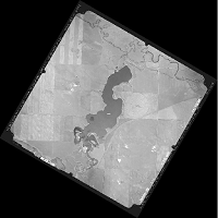
-
The surveys are conducted along the sandspit and within a 96 ha lagoon that encompasses mudflats, eelgrass beds, and saltmarsh at the northwest end of Sidney Island, located in the Strait of Georgia, British Columbia. The survey counts numerate two species, Western Sandpiper (Calidris mauri) and Least Sandpiper (Calidris minutilla), during a portion of the southern migration period (July, August, and early September), and have been conducted intermittently since 1990. Sidney Island (48°37’39’N, 123°19’30”W) is located within the Salish Sea (Strait of Georgia), 4 km off the coast of Vancouver Island in southwestern British Columbia, Canada. Southbound Western and Least Sandpipers stop over within Sidney Spit Marine Park (part of the Gulf Islands National Park Reserve), roosting and feeding along the sandspit and within a 96 ha lagoon that encompasses mudflats, eelgrass beds, and saltmarsh at the northwest end of the island. These species are the most numerous shorebird species using the area during southern migration. Adults precede juveniles, arriving at the end of June and throughout July. Juveniles reach the site in early August, with their numbers trailing off in early September. As a result, the site experiences a transition from purely adult to purely juvenile flocks over the course of the season. Daily counts, beginning in early July and ending in early September, were conducted in 1990 and from 1992-2001 (no counts occurred in 1991). Effort was reduced to weekly surveys between 2002 and 2013. Over the entire monitoring period median survey effort was 9 counts annually. All counts were conducted at the low tide of the day, when shorebirds were feeding in the exposed mudflat of the lagoon. Observers walked along the shore of the lagoon stopping periodically at vantage points to look for birds. For ease of data recording and to keep track of individual flocks, the survey area was divided into separate units demarcated by prominent geographical features. Counts were made with the unaided eye, through binoculars, and with a 20 – 60x zoom spotting scope, depending on the proximity of the birds. All individuals in small flocks were counted and individuals in large flocks were estimated by counting in groups of 5, 10, 50 or 100 according to flock size in each successive field of view across a scan of the entire flock. Between 1990 and 2001, when daily counts were conducted, birds were occasionally counted more than once in a day. The largest count value obtained was used as the daily estimate for these days. For smaller flocks, we were able to identify all individual birds to species and age-class. Sub-samples from larger flocks were also aged (adult or juvenile) and identified to species. Birds were aged by plumage characteristics. Adult Western Sandpipers are distinguished from juveniles by the dark chevron markings present along the sides and breast. Juvenile Least Sandpipers have a buffy breast compared to the distinct, darker one of the adult, and juveniles have bright rufous scapulars compared to the drab feather-edges of the adults. In both species, juvenile plumage appears brighter and cleaner than adult plumage, which is more worn and tattered.
-
Multi-model ensembles of mean temperature based on projections from twenty-nine Coupled Model Intercomparison Project Phase 5 (CMIP5) global climate models are available for 1901-2100. Specifically, the 5th, 25th, 50th, 75th and 95th percentiles of the monthly, seasonal and annual ensembles of mean temperature (°C) are available for the historical time period, 1901-2005, and for emission scenarios, RCP2.6, RCP4.5 and RCP8.5, for 2006-2100. Note: Projections among climate models can vary because of differences in their underlying representation of earth system processes. Thus, the use of a multi-model ensemble approach has been demonstrated in recent scientific literature to likely provide better projected climate change information.