 Arctic SDI catalogue
series
Type of resources
Available actions
Topics
Keywords
Contact for the resource
Provided by
Years
Formats
Representation types
Scale
Resolution
-
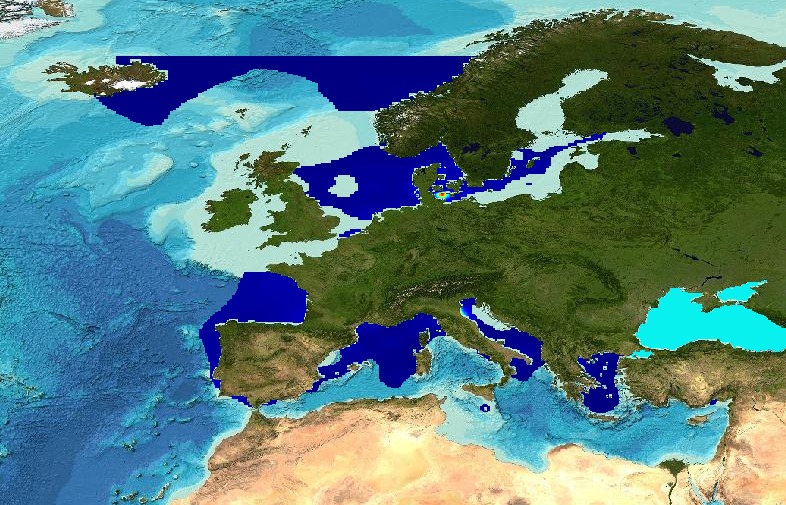
Moving 6-year analysis and visualization of Water body silicate in the North Sea. Four seasons (December-February, March-May, June-August, September-November). Data Sources: observational data from SeaDataNet/EMODnet Chemistry Data Network. Description of DIVA analysis: Geostatistical data analysis by DIVAnd (Data-Interpolating Variational Analysis) tool, version 2.7.9. results were subjected to the minfield option in DIVAnd to avoid negative/underestimated values in the interpolated results; error threshold masks L1 (0.3) and L2 (0.5) are included as well as the unmasked field. The depth dimension allows visualizing the gridded field at various depths.
-
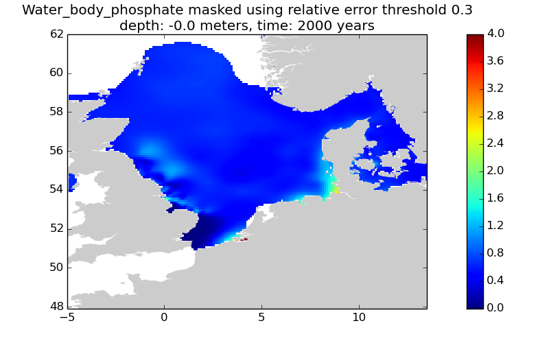
This gridded product visualizes 1960 - 2014 water body phosphate concentration (umol/l) in the North Sea domain, for each season (winter: December – February; spring: March – May; summer: June – August; autumn: September – November). It is produced as a Diva 4D analysis, version 4.6.9: a reference field of all seasonal data between 1960-2014 was used; results were logit transformed to avoid negative/underestimated values in the interpolated results; error threshold masks L1 (0.3) and L2 (0.5) are included as well as the unmasked field. Every step of the time dimension corresponds to a 10-year moving average for each season. The depth dimension allows visualizing the gridded field at various depths.
-
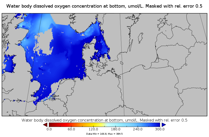
This gridded product visualizes 1960 - 2014 water body dissolved oxygen concentration (umol/l) in the North Sea domain, for each season (winter: December – February; spring: March – May; summer: June – August; autumn: September – November). It is produced as a Diva 4D analysis, version 4.6.11: a reference field of all seasonal data between 1960-2014 was used; results were logit transformed to avoid negative/underestimated values in the interpolated results; error threshold masks L1 (0.3) and L2 (0.5) are included as well as the unmasked field. Every step of the time dimension corresponds to a 10-year moving average for each season. The depth dimension allows visualizing the gridded field at various depths.
-
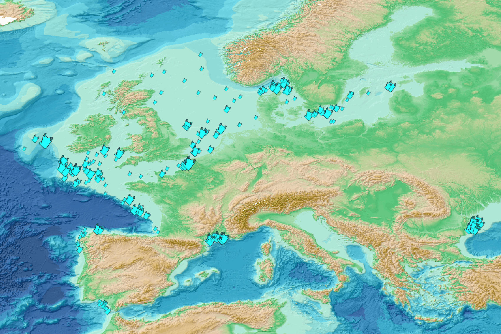
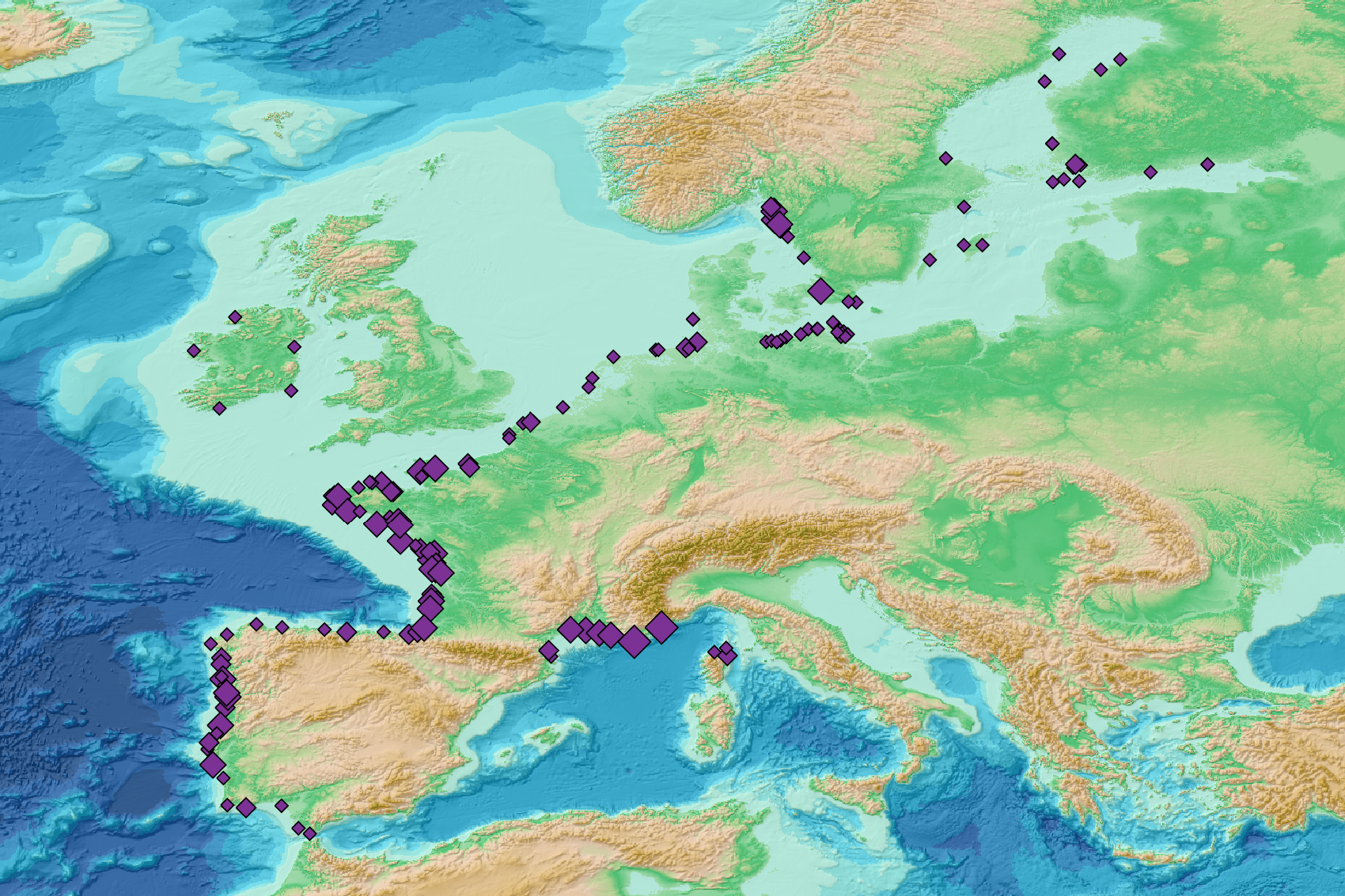
This visualization product displays plastic bags density per trawl. EMODnet Chemistry included the collection of marine litter in its 3rd phase. Since the beginning of 2018, data of seafloor litter collected by international fish-trawl surveys have been gathered and processed in the EMODnet Chemistry Marine Litter Database (MLDB). The harmonization of all the data has been the most challenging task considering the heterogeneity of the data sources, sampling protocols (OSPAR and MEDITS protocols) and reference lists used on a European scale. Moreover, within the same protocol, different gear types are deployed during fishing bottom trawl surveys. In cases where the wingspread and/or number of items were unknown, data could not be used because these fields are needed to calculate the density. Data collected before 2011 are affected by this filter. When the distance reported in the data was null, it was calculated from: - the ground speed and the haul duration using this formula: Distance (km) = Haul duration (h) * Ground speed (km/h); - the trawl coordinates if the ground speed and the haul duration were not filled in. The swept area is calculated from the wingspread (which depends on the fishing gear type) and the distance trawled: Swept area (km²) = Distance (km) * Wingspread (km) Densities have been calculated on each trawl and year using the following computation: Density of plastic bags (number of items per km²) = ∑Number of plastic bags related items / Swept area (km²) Percentiles 50, 75, 95 & 99 have been calculated taking into account data for all years. The list of selected items for this product is attached to this metadata. Information on data processing and calculation is detailed in the attached methodology document. Warning: the absence of data on the map doesn't necessarily mean that they don't exist, but that no information has been entered in the Marine Litter Database for this area.
-
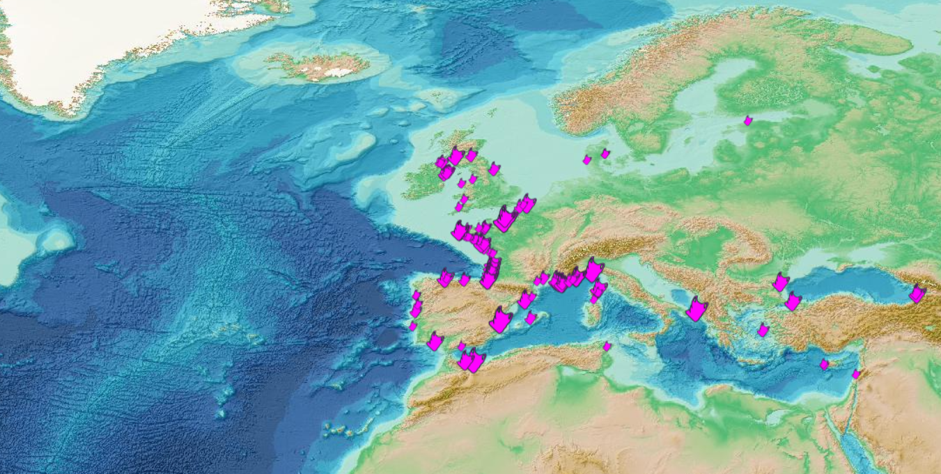
This visualization product displays the number of Marine Strategy Framework Directive (MSFD) monitoring surveys and the associated temporal coverage per beach. EMODnet Chemistry included the collection of marine litter in its 3rd phase. Since the beginning of 2018, data of beach litter have been gathered and processed in the EMODnet Chemistry Marine Litter Database (MLDB). The harmonization of all the data has been the most challenging task considering the heterogeneity of the data sources, sampling protocols and reference lists used on a European scale. Preliminary processings were necessary to harmonize all the data: - Exclusion of OSPAR 1000 protocol: in order to follow the approach of OSPAR that it is not including these data anymore in the monitoring; - Selection of MSFD surveys only (exclusion of other monitoring, cleaning and research operations); - Exclusion of beaches without coordinates. More information is available in the attached documents. Warning: the absence of data on the map does not necessarily mean that they do not exist, but that no information has been entered in the Marine Litter Database for this area.
-

This visualization product displays the cigarette related items abundance of marine macro-litter (> 2.5cm) per beach per year from Marine Strategy Framework Directive (MSFD) monitoring surveys without UNEP-MARLIN data. EMODnet Chemistry included the collection of marine litter in its 3rd phase. Since the beginning of 2018, data of beach litter have been gathered and processed in the EMODnet Chemistry Marine Litter Database (MLDB). The harmonization of all the data has been the most challenging task considering the heterogeneity of the data sources, sampling protocols and reference lists used on a European scale. Preliminary processings were necessary to harmonize all the data: - Exclusion of OSPAR 1000 protocol: in order to follow the approach of OSPAR that it is not including these data anymore in the monitoring; - Selection of MSFD surveys only (exclusion of other monitoring, cleaning and research operations); - Exclusion of beaches without coordinates; - Selection of cigarette related items only. The list of selected items is attached to this metadata. This list was created using EU Marine Beach Litter Baselines, the European Threshold Value for Macro Litter on Coastlines and the Joint list of litter categories for marine macro-litter monitoring from JRC (these three documents are attached to this metadata); - Exclusion of surveys referring to the UNEP-MARLIN list: the UNEP-MARLIN protocol differs from the other types of monitoring in that cigarette butts are surveyed in a 10m square. To avoid comparing abundances from very different protocols, the choice has been made to distinguish in two maps the cigarette related items results associated with the UNEP-MARLIN list from the others; - Normalization of survey lengths to 100m & 1 survey / year: in some case, the survey length was not exactly 100m, so in order to be able to compare the abundance of litter from different beaches a normalization is applied using this formula: Number of cigarette related items of the survey (normalized by 100 m) = Number of cigarette related items of the survey x (100 / survey length) Then, this normalized number of cigarette related items is summed to obtain the total normalized number of cigarette related items for each survey. Finally, the median abundance of cigarette related items for each beach and year is calculated from these normalized abundances of cigarette related items per survey. Sometimes the survey length was null or equal to 0. Assuming that the MSFD protocol has been applied, the length has been set at 100m in these cases. Percentiles 50, 75, 95 & 99 have been calculated taking into account cigarette related items from MSFD monitoring data (excluding UNEP-MARLIN protocol) for all years. More information is available in the attached documents. Warning: the absence of data on the map does not necessarily mean that they do not exist, but that no information has been entered in the Marine Litter Database for this area.
-
The analysis was performed per season using DIVA software tool (Data-Interpolating Variational Analysis). The analyses products are stored as NetCDF CF files and made available as WMS layers for easy browsing and adding. Every step of the time dimension corresponds to a 6-year moving average from 1983 to 2016. The depth dimension spans from surface to 1000 m, with 21 vertical levels. The boundaries and overlapping zones between these regions were filtered to avoid any unrealistic spatial discontinuities. This combined water body dissolved oxygen concentration product is masked using the relative error threshold 0.5. Units: µmol/l Created by 'University of Liège, GeoHydrodynamics and Environment Research (ULiège-GHER)'. The data used as input for DIVA have been extracted from the EMODnet Chemistry Download Service: https://emodnet-chemistry.maris.nl/search Intermediate regional data products: Mediterranean Sea - DIVA 4D 6-year analysis of Water body chlorophyll-a 1990/2017 v2018, Arctic Ocean - DIVA 4D 6-year analysis of Water body chlorophyll-a 1980/2017 v2018, Black Sea - DIVA 4D 6-year analysis of Water body chlorophyll-a 1990/2016 v2018, North East Atlantic Ocean - DIVA 4D 6-year analysis of Water body chlorophyll-a 1960/2017 v2018, North Sea - DIVA 4D 6-year analysis of Water body chlorophyll-a 1980/2017 v2018, Baltic Sea - DIVA 4D 6-year analysis of Water body chlorophyll-a 1980/2016 v2018
-
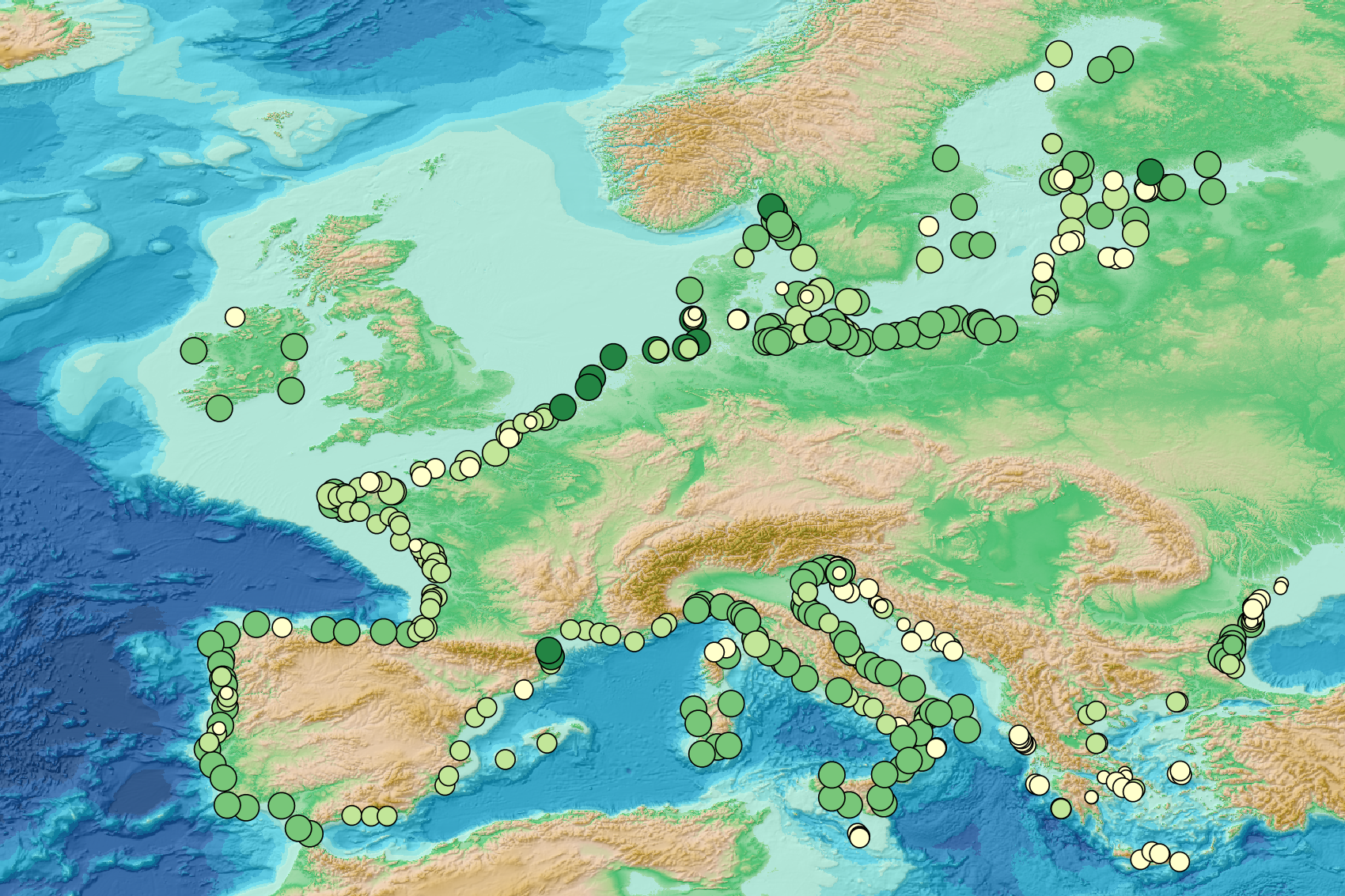
This visualization product displays the total abundance of marine macro-litter (> 2.5cm) per beach per year from Marine Strategy Framework Directive (MSFD) monitoring surveys. EMODnet Chemistry included the collection of marine litter in its 3rd phase. Since the beginning of 2018, data of beach litter have been gathered and processed in the EMODnet Chemistry Marine Litter Database (MLDB). The harmonization of all the data has been the most challenging task considering the heterogeneity of the data sources, sampling protocols and reference lists used on a European scale. Preliminary processings were necessary to harmonize all the data: - Exclusion of OSPAR 1000 protocol: in order to follow the approach of OSPAR that it is not including these data anymore in the monitoring; - Selection of MSFD surveys only (exclusion of other monitoring, cleaning and research operations); - Exclusion of beaches without coordinates; - Some categories & some litter types like organic litter, small fragments (paraffin and wax; items > 2.5cm) and pollutants have been removed. The list of selected items is attached to this metadata. This list was created using EU Marine Beach Litter Baselines, the European Threshold Value for Macro Litter on Coastlines and the Joint list of litter categories for marine macro-litter monitoring from JRC (these three documents are attached to this metadata); - Normalization of survey lengths to 100m & 1 survey / year: in some cases, the survey length was not exactly 100m, so in order to be able to compare the abundance of litter from different beaches a normalization is applied using this formula: Number of items (normalized by 100 m) = Number of litter per items x (100 / survey length) Then, this normalized number of items is summed to obtain the total normalized number of litter for each survey. Finally, the median abundance for each beach and year is calculated from these normalized abundances per survey. Sometimes the survey length was null or equal to 0. Assuming that the MSFD protocol has been applied, the length has been set at 100m in these cases. Percentiles 50, 75, 95 & 99 have been calculated taking into account MSFD data for all years. More information is available in the attached documents. Warning: the absence of data on the map does not necessarily mean that it does not exist, but that no information has been entered in the Marine Litter Database for this area.
-
This visualization product displays the plastic bags abundance of marine macro-litter (> 2.5cm) per beach per year from non-MSFD monitoring surveys, research & cleaning operations. EMODnet Chemistry included the collection of marine litter in its 3rd phase. Since the beginning of 2018, data of beach litter have been gathered and processed in the EMODnet Chemistry Marine Litter Database (MLDB). The harmonization of all the data has been the most challenging task considering the heterogeneity of the data sources, sampling protocols and reference lists used on a European scale. Preliminary processing were necessary to harmonize all the data: - Exclusion of OSPAR 1000 protocol: in order to follow the approach of OSPAR that it is not including these data anymore in the monitoring; - Selection of surveys from non-MSFD monitoring, cleaning and research operations; - Exclusion of beaches without coordinates; - Selection of plastic bags related items only. The list of selected items is attached to this metadata. This list was created using EU Marine Beach Litter Baselines and EU Threshold Value for Macro Litter on Coastlines from JRC (these two documents are attached to this metadata); - Exclusion of surveys without associated length; - Normalization of survey lengths to 100m & 1 survey / year: in some case, the survey length was not 100m, so in order to be able to compare the abundance of litter from different beaches a normalization is applied using this formula: Number of plastic bags related items of the survey (normalized by 100 m) = Number of plastic bags related items of the survey x (100 / survey length) Then, this normalized number of plastic bags related items is summed to obtain the total normalized number of plastic bags related items for each survey. Finally, the median abundance of plastic bags related items for each beach and year is calculated from these normalized abundances of plastic bags related items per survey. Percentiles 50, 75, 95 & 99 have been calculated taking into account plastic bags related items from other sources data for all years. More information is available in the attached documents. Warning: the absence of data on the map doesn't necessarily mean that they don't exist, but that no information has been entered in the Marine Litter Database for this area.
-
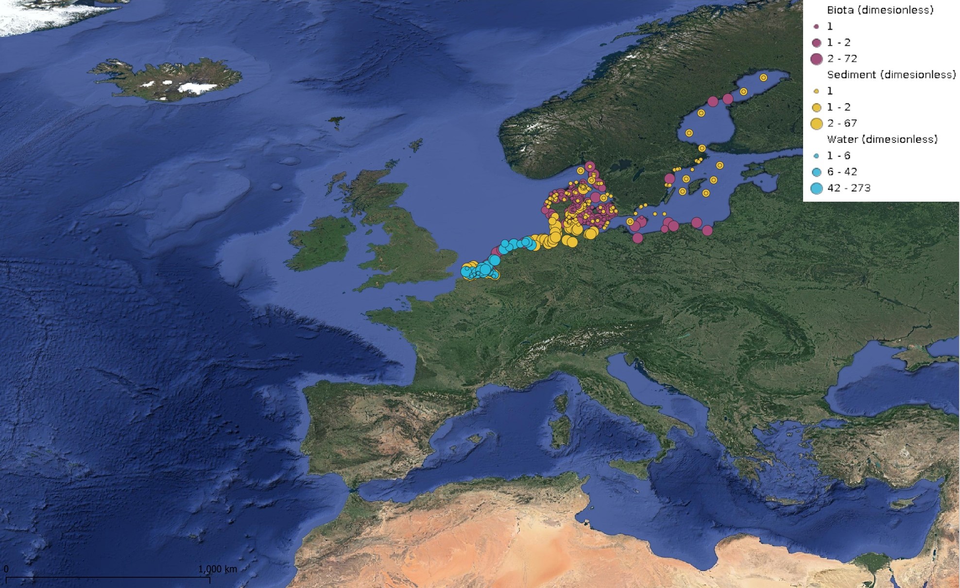
This product displays for Triphenyltin, positions with values counts that have been measured per matrix and are present in EMODnet regional contaminants aggregated datasets, v2024. The product displays positions for all available years.