 Arctic SDI catalogue
marine
Type of resources
Available actions
Topics
Keywords
Contact for the resource
Provided by
Years
Formats
Representation types
Update frequencies
status
Service types
Scale
-
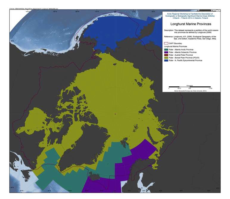
This dataset represents a partition of the world oceans into provinces as defined by Longhurst (1995; 1998; 2006), and are based on the prevailing role of physical forcing as a regulator of phytoplankton distribution. The dataset represents the initial static boundaries developed at the Bedford Institute of Oceanography, Canada. Note that the boundaries of these provinces are not fixed in time and space, but are dynamic and move under seasonal and interannual changes in physical forcing. At the first level of reduction, Longhurst recognized four principal biomes (also referred to as domains in earlier publications): the Polar Biome, the Westerlies Biome, the Trade-Winds Biome, and the Coastal Boundary Zone Biome. These four Biomes are recognizable in every major ocean basin. At the next level of reduction, the ocean basins are partitioned into provinces, roughly ten for each basin. These partitions provide a template for data analysis or for making parameter assignments on a global scale. (source: VLIZ (2009). Longhurst Biogeographical Provinces. Available online at <a href="http://www.marineregions.org/" target="_blank">Longhurst Biogeographical Provinces</a> References: Longhurst, A.R. (2006). Ecological Geography of the Sea. 2nd Edition. Academic Press, San Diego, 560p. Data available from: <a href="http://www.marineregions.org/sources.php#longhurst" target="_blank">Ecological Geography of the Sea</a>
-
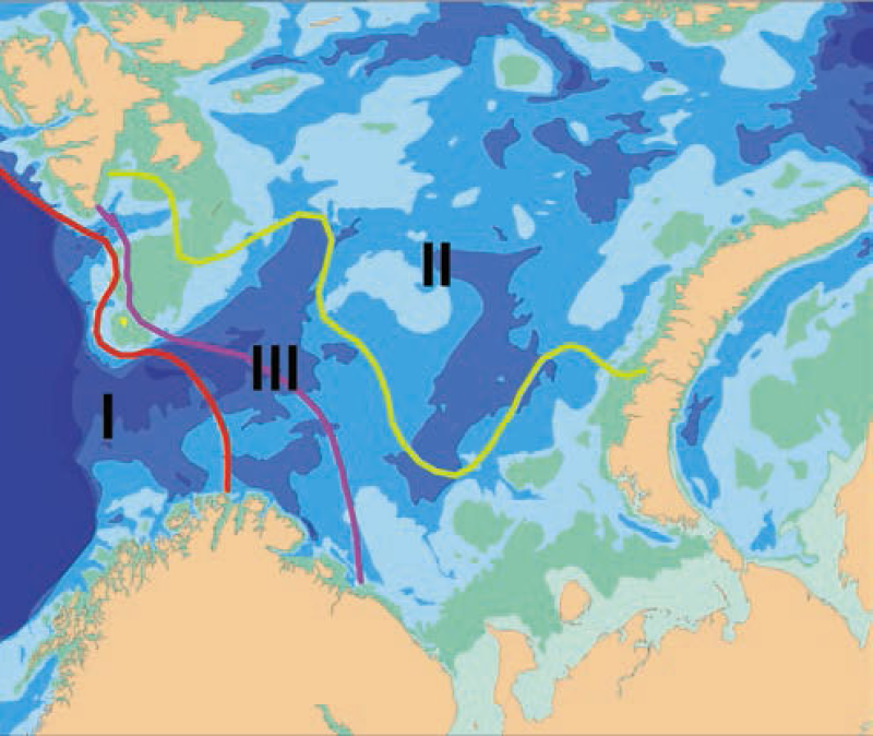
Biogeographic borders in the Barents Sea based on species distributions of bryozoans. Average position of the border with 50:50% of Atlantic boreal and Arctic species numbers is indicated by the pink line, and the red and green lines indicate the extreme positions of the border in cold and warm periods respectively. Area III between them is the transitional zone between the Atlantic boreal and the Arctic regions. Thus, area I always has > 50% Atlantic boreal species, and area II always > 50% Arctic species (after Denisenko 1990).
-
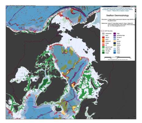
We present the first digital seafloor geomorphic features map (GSFM) of the global ocean. The GSFM includes 131,192 separate polygons in 29 geomorphic feature categories, used here to assess differences between passive and active continental margins as well as between 8 major ocean regions (the Arctic, Indian, North Atlantic, North Pacific, South Atlantic, South Pacific and the Southern Oceans and the Mediterranean and Black Seas). The GSFM provides quantitative assessments of differences between passive and active margins: continental shelf width of passive margins (88 km) is nearly three times that of active margins (31 km); the average width of active slopes (36 km) is less than the average width of passive margin slopes (46 km); active margin slopes contain an area of 3.4 million km2 where the gradient exceeds 5°, compared with 1.3 million km2 on passive margin slopes; the continental rise covers 27 million km2 adjacent to passive margins and less than 2.3 million km2 adjacent to active margins. Examples of specific applications of the GSFM are presented to show that: 1) larger rift valley segments are generally associated with slow-spreading rates and smaller rift valley segments are associated with fast spreading; 2) polar submarine canyons are twice the average size of non-polar canyons and abyssal polar regions exhibit lower seafloor roughness than non-polar regions, expressed as spatially extensive fan, rise and abyssal plain sediment deposits – all of which are attributed here to the effects of continental glaciations; and 3) recognition of seamounts as a separate category of feature from ridges results in a lower estimate of seamount number compared with estimates of previous workers. Reference: Harris PT, Macmillan-Lawler M, Rupp J, Baker EK Geomorphology of the oceans. Marine Geology.
-
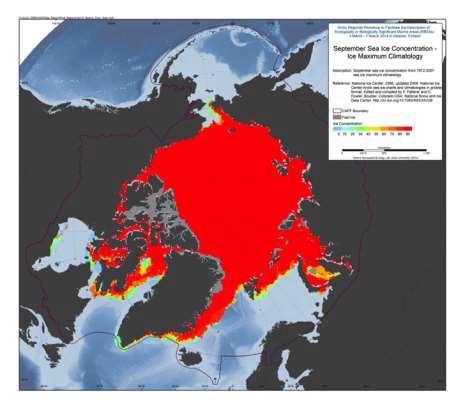
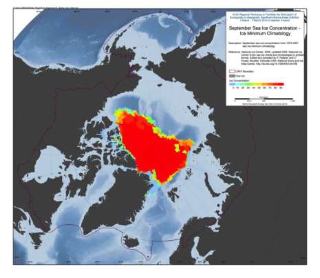
The U.S. National Ice Center (NIC) is an inter-agency sea ice analysis and forecasting center comprised of the Department of Commerce/NOAA, the Department of Defense/U.S. Navy, and the Department of Homeland Security/U.S. Coast Guard components. Since 1972, NIC has produced Arctic and Antarctic sea ice charts. This data set is comprised of Arctic sea ice concentration climatology derived from the NIC weekly or biweekly operational ice-chart time series. The charts used in the climatology are from 1972 through 2007; and the monthly climatology products are median, maximum, minimum, first quartile, and third quartile concentrations, as well as frequency of occurrence of ice at any concentration for the entire period of record as well as for 10-year and 5-year periods. NIC charts are produced through the analyses of available in situ, remote sensing, and model data sources. They are generated primarily for mission planning and safety of navigation. NIC charts generally show more ice than do passive microwave derived sea ice concentrations, particularly in the summer when passive microwave algorithms tend to underestimate ice concentration. The record of sea ice concentration from the NIC series is believed to be more accurate than that from passive microwave sensors, especially from the mid-1990s on (see references at the end of this documentation), but it lacks the consistency of some passive microwave time series. Source: <a href="http://nsidc.org/data/G02172" target="_blank">NSIDC</a> Reference: National Ice Center. 2006, updated 2009. National Ice Center Arctic sea ice charts and climatologies in gridded format. Edited and compiled by F. Fetterer and C. Fowler. Boulder, Colorado USA: National Snow and Ice Data Center. Source: <a href="http://nsidc.org/data/G02172" target="_blank">NSIDC</a>
-
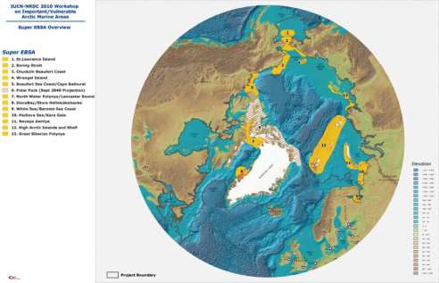
The International Union for the Conservation of Nature (IUCN) and the Natural Resources Defense Council (NRDC) have undertaken a project to explore ways of advancing implementation of ecosystem- based management in the Arctic marine environment through invited expert workshops. The first workshop, held in Washington, D.C. on 16-18 June, 2010, explored possible means to advance policy decisions on ecosystem-based marine management in the Arctic region. Twentynine legal and policy experts from around the region participated in the June workshop. The report and recommendations of the June policy workshop can be found here: <a href="http://cmsdata.iucn.org/downloads/arctic_workshop_report_final.pdf" target="_blank">Workshop report</a> The second workshop, the subject of this report, was held at the Scripps Institution of Oceanography in La Jolla, California on 2-4 November, 2010. The La Jolla workshop utilized criteria developed under auspices of the Convention on Biological Diversity to identify ecologically significant and vulnerable marine areas that should be considered for enhanced protection in any new ecosystem-based management arrangements. A list of participants, the meeting agenda and other relevant documents are attached as appendices to this repor, see: <a href="https://www.nrdc.org/sites/default/files/oce_11042501a.pdf" target="_blank">Workshop report</a>
-
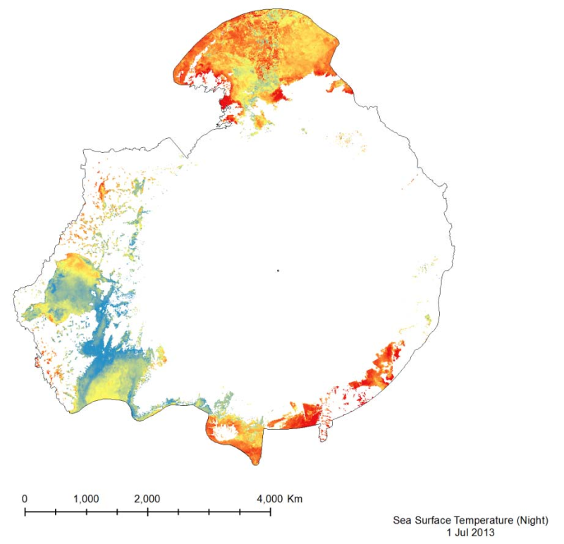
The MODIS Sea Surface Temperature (SST) product provided is a 4km spatialresolution monthly composite made from nighttime measurements from the Aqua Satellite.The nighttime measurements are used to collect a consistent temperature measurement that isunaffected by the warming of the top layer of water by the sun.
-
The U.S. National Ice Center (NIC) is an inter-agency sea ice analysis and forecasting center comprised of the Department of Commerce/NOAA, the Department of Defense/U.S. Navy, and the Department of Homeland Security/U.S. Coast Guard components. Since 1972, NIC has produced Arctic and Antarctic sea ice charts. This data set is comprised of Arctic sea ice concentration climatology derived from the NIC weekly or biweekly operational ice-chart time series. The charts used in the climatology are from 1972 through 2007; and the monthly climatology products are median, maximum, minimum, first quartile, and third quartile concentrations, as well as frequency of occurrence of ice at any concentration for the entire period of record as well as for 10-year and 5-year periods. NIC charts are produced through the analyses of available in situ, remote sensing, and model data sources. They are generated primarily for mission planning and safety of navigation. NIC charts generally show more ice than do passive microwave derived sea ice concentrations, particularly in the summer when passive microwave algorithms tend to underestimate ice concentration. The record of sea ice concentration from the NIC series is believed to be more accurate than that from passive microwave sensors, especially from the mid-1990s on (see references at the end of this documentation), but it lacks the consistency of some passive microwave time series. Source: <a href="http://nsidc.org/data/G02172" target="_blank">NSIDC</a> Reference: National Ice Center. 2006, updated 2009. National Ice Center Arctic sea ice charts and climatologies in gridded format. Edited and compiled by F. Fetterer and C. Fowler. Boulder, Colorado USA: National Snow and Ice Data Center. Source: <a href="http://nsidc.org/data/G02172" target="_blank">NSIDC</a>
-
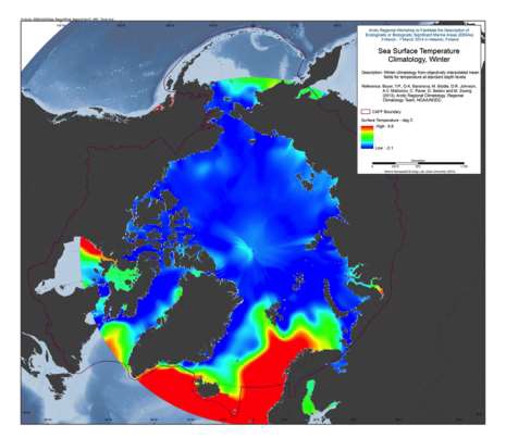
A set of mean fields for temperature and salinity for the Arctic Seas and environs are available for viewing and downloading. Area: The area encompassed is all longitudes from 60°N to 90°N latitudes. Horizontal resolution: Temperature and salinity are available on a 1°x1° and a 1/4°x1/4° latitude/longitude grid. Time resolution: All climatologies for all variables use all available data regardless of year of measurement. Climatologies were calculated for annual (all-data), seasonal, and monthly time periods. Seasons are as follows: Winter (Jan.-Mar.), Spring (Apr.-Jun.), Summer (Jul.-Aug.), Fall (Oct.-Dec.). Vertical resolution: Temperature and salinity are available on 87 standard levels with higher vertical resolution than the World Ocean Atlas 2009 (WOA09), but levels extend from the surface to 4000 m. Units: Temperature units are °C. Salinity is unitless on the Practical Salinity Scale-1978 [PSS]. Data used: All data from the area found in the World Ocean Database (WOD) as of the end of 2011. For a description of this dataset, please see World Ocean Database 2009 IntroductionMethod: The method followed for calculation of the mean climatological fields is detailed in the following publications: Temperature: Locarnini et al., 2010, Salinity: Antonov et al., 2010. Additional details on the 1/4° climatological calculation are found in Boyer et al., 2005, from: <a href="http://www.nodc.noaa.gov/OC5/regional_climate/arctic/" target="_blank">NOAA</a> Reference: Boyer, T.P., O.K. Baranova, M. Biddle, D.R. Johnson, A.V. Mishonov, C. Paver, D. Seidov and M. Zweng (2012), Arctic Regional Climatology, Regional Climatology Team, NOAA/NODC, source: <a href="www.nodc.noaa.gov/OC5/regional_climate/arctic" target="_blank">NOAA</a>
-
In the Marine Strategy Framework Directive (MSFD), four marine regions are listed (art. 4). The North-east Atlantic Ocean and Mediterranean Sea marine regions are both further divided into four subregions. The marine regions and subregions include: The Baltic SeaThe North-east Atlantic OceanThe Greater North Sea, including the Kattegat and the English ChannelThe Celtic SeasThe Bay of Biscay and the Iberian CoastMacaronesiaThe Mediterranean SeaThe Western Mediterranean SeaThe Adriatic SeaThe Ionian Sea and the Central Mediterranean SeaThe Aegean-Levantine SeaThe Black SeaThis map has been developed to support DG Environment and EU Member States in their implementation of the MSFD. It represents the current state of understanding of the marine regions and subregions and is subject to amendment in light of any new information which may be received.The primary aim of this map is the geometric delineation of the marine regions and subregions. The secondary aim is to establish a common understanding of marine boundaries and thus aid the streamlining of obligations under EU legislation, e.g. coordination between Member States, work establishment of monitoring programmes, establishment of programmes of measures, EEA indicator and assessment efforts and ‘Research and Technological Development’ (RTD) initiatives to be as relevant as possible for policy processes aiming at implementing an ecosystem-based approach to management. Lastly, the map can aid the harmonization between regions as required under other EU legislation and policies, by Regional Sea Conventions, International Council for the Exploration of the Sea (ICES) Ecoregions and other regional delineations. The aim is not to pre-empt any official discussions on maritime boundaries under UNCLOS.The delineation has been developed since 2010 based on multiple inputs from Member State representatives participating in groups defined under the MSFD Common Implementation Strategy, reporting under the MSFD Initial Assessment, ICES advice and Marine Regions. The process has especially been developed under the MSFD CIS Working Group on Data, Information and Knowledge Exchange (WGDIKE) through documents DIKE 3/2011/06 from 5-6thSeptember 2011, DIKE 4/2011/05 from 7-8thNovember 2011, DIKE 5/2012/08 from 12-13thMarch 2012, DIKE TG1/2012/04 from 4thJuly 2012 and, lastly, DIKE 6/2012/11 from 30-31th October 2012. Since then it has been developed through cooperation between DG ENV, EEA and the ETC-ICM (via ICES as an ETC-ICM partner) and a consultation with Member States in 2015. The map has also been through a Commission inter-service consultation with all DG’s led by DG ENV. It wasfinallyadopted by EU Member States in the MSFD Committee in November 2016. The boundaries between marine regions and subregions have, to the extent possible, been harmonised with existing boundaries established under the Regional Sea Conventions, the biogeographic boundaries established under the Habitats Directive and the boundaries of marine waters reported by EU Member States under the MSFD. The ICES ecoregions are being aligned with the MSFD region and subregion boundaries.The inner boundary of all regions and subregions has used the “EEA coastline for analysis” available at (http://www.eea.europa.eu/data-and-maps/data/eea-coastline-for-analysis/); this is a practical solution because the MSFD inner boundary formally follows that defined for coastal waters under the Water Framework Directive, for which a consistent boundary is not yet available.For delineating subregions in the North-east Atlantic Ocean region, information on Member States' marine waters, where Member States have and/or exercise jurisdictional rights, has been used, based on submissions of the marine waters under the MSFD when these have been made available by the individual Member States as part of their 2012 reporting.Regarding the map symbology, the following notes have to be taken into account:Note 1:The area shaded in purple and white indicates an area to which both the United Kingdom and the Government of the Kingdom of Denmark together with the Government of the Faroes have transmitted overlapping submissions to the Commission on the Limits of the Continental Shelf (CLCS) in fulfilment of their respective rights and obligations under Article 76 and Annex II to the United Nations Convention on the Law of the Sea in order to determine entitlement of outer continental shelf areas. This map should not be used in any way to prejudice the determination of that question by the CLCS in due course.Note 2:The area shaded in black and white shows the delineation of the outer limits of the continental shelf beyond 200 M from the territorial sea baselines of France, Ireland, Spain and the United Kingdom in respect of the area of the Celtic Sea and the Bay of Biscay, as provided by the four countries to the Commission on the Limits of the Continental Shelf (CLCS) and included in its recommendations issued on 24 March 2009. The map of the continental shelf’s extent shall be used without prejudice to the agreements that will be concluded in due course between these Member States on their marine borders in this area.Note 3: The seas of Azov and Marmara are shown as shaded as they do not fall within the geographic scope of application of the Bucharest Convention.The link to the layers, as well as the document describingthe geometric delineation of the marine regions and subregionsandthe process that led to an agreement on the boundaries areavailable at the following link: http://www.eea.europa.eu/data-and-maps/data/msfd-regions-and-subregions
-

The U.S. National Ice Center (NIC) is an inter-agency sea ice analysis and forecasting center comprised of the Department of Commerce/NOAA, the Department of Defense/U.S. Navy, and the Department of Homeland Security/U.S. Coast Guard components. Since 1972, NIC has produced Arctic and Antarctic sea ice charts. This data set is comprised of Arctic sea ice concentration climatology derived from the NIC weekly or biweekly operational ice-chart time series. The charts used in the climatology are from 1972 through 2007; and the monthly climatology products are median, maximum, minimum, first quartile, and third quartile concentrations, as well as frequency of occurrence of ice at any concentration for the entire period of record as well as for 10-year and 5-year periods. NIC charts are produced through the analyses of available in situ, remote sensing, and model data sources. They are generated primarily for mission planning and safety of navigation. NIC charts generally show more ice than do passive microwave derived sea ice concentrations, particularly in the summer when passive microwave algorithms tend to underestimate ice concentration. The record of sea ice concentration from the NIC series is believed to be more accurate than that from passive microwave sensors, especially from the mid-1990s on (see references at the end of this documentation), but it lacks the consistency of some passive microwave time series. Source: <a href="http://nsidc.org/data/G02172" target="_blank">NSIDC</a> Reference: National Ice Center. 2006, updated 2009. National Ice Center Arctic sea ice charts and climatologies in gridded format. Edited and compiled by F. Fetterer and C. Fowler. Boulder, Colorado USA: National Snow and Ice Data Center. Source: <a href="http://nsidc.org/data/G02172" target="_blank">NSIDC</a>