 Arctic SDI catalogue
External Authoritative
Type of resources
Available actions
Topics
Keywords
Contact for the resource
Provided by
Years
Formats
Service types
Scale
Resolution
-
Different dataset added toghether to make a common database for the workshop in Oslo and for the upcoming worskhop on Crete. Investigate biodiversity across Europe: The database consist of bottom-dwelling macro benthos collected in Arctic (Franz Josef Land, Pechora Sea, Svalbard),along the Norwegian Continental Shelf, in Irish Sea, Ionan Sea, Aegean Sea, and the Black Sea. 3,616 taxa and 1,064,225 individuals including 26,313 juvenile in 1,243 sediment samples. Equipment Surface (m2) Samples Replicates Van Veen Grab 0.1 518 2 – 5 grabs, mostly 5. Van Veen Grab 0.04 33 1 Ponar Grab 0.05 39 1 Ocean Grab 0.25 50 1 Boxcorer 0.25 16 2 Hand-operated Van Veen Grab 0.08 18 1 Hand operated van Veen Grab 0.05 64 1 Hand operated grab type Ponar 0.045 70 1 Hand operated Smith-McIntyre sampler 0.1 14 1 Hand operated van Veen Grab; Scuba diving; Free diving; Otter trawl - 421 “p/a” 1937 – 2000
-
Moving 6-year analysis and visualization of Water body silicate in the North Sea. Four seasons (December-February, March-May, June-August, September-November). Data Sources: observational data from SeaDataNet/EMODnet Chemistry Data Network. Description of DIVA analysis: Geostatistical data analysis by DIVAnd (Data-Interpolating Variational Analysis) tool, version 2.7.9. results were subjected to the minfield option in DIVAnd to avoid negative/underestimated values in the interpolated results; error threshold masks L1 (0.3) and L2 (0.5) are included as well as the unmasked field. The depth dimension allows visualizing the gridded field at various depths.
-

The Rolling Archive database (WLRA) is one of the products of the pan-European High-Resolution Water Snow & Ice portfolio (HR-WSI), which are provided at high spatial resolution from the Sentinel-2 and Sentinel-1 constellations data from September 1, 2016 onwards. The High Resolution Water Layer portfolio consists of the Water Layer (WL), the Water Presence Index (WPI), the Water confidence layer (WCL) and the Rolling archive (WLRA). The WLRA consists of intermediate production layers such as water and wetness masks showing the seasonal water and dry occurrences starting 2009. The masks are used for the generation of the Water Layer which covers a period of seven years per reference year and is regularly updated every three years. It is therefore important that it is consistent over the entire period. To guarantee reproducibility and future continuation of the baseline product, these masks are provided within a database consisting of all seasonal masks starting from 2009. With the new update of the Water product, the HR WL for the reference year 2021 only water masks will be continued. Additionally, the computation frequency changed from seasonal to monthly masks. This update covers a period from 2016.09.01 to 20211231 including an update of the masks already availbe from the historic 2018 production. The binary masks are provided across Europe in a spatial resolution of 10 m x 10 m as GeoTiffs zipped in a ZARR file.
-
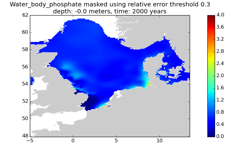
This gridded product visualizes 1960 - 2014 water body phosphate concentration (umol/l) in the North Sea domain, for each season (winter: December – February; spring: March – May; summer: June – August; autumn: September – November). It is produced as a Diva 4D analysis, version 4.6.9: a reference field of all seasonal data between 1960-2014 was used; results were logit transformed to avoid negative/underestimated values in the interpolated results; error threshold masks L1 (0.3) and L2 (0.5) are included as well as the unmasked field. Every step of the time dimension corresponds to a 10-year moving average for each season. The depth dimension allows visualizing the gridded field at various depths.
-
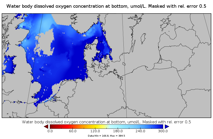
This gridded product visualizes 1960 - 2014 water body dissolved oxygen concentration (umol/l) in the North Sea domain, for each season (winter: December – February; spring: March – May; summer: June – August; autumn: September – November). It is produced as a Diva 4D analysis, version 4.6.11: a reference field of all seasonal data between 1960-2014 was used; results were logit transformed to avoid negative/underestimated values in the interpolated results; error threshold masks L1 (0.3) and L2 (0.5) are included as well as the unmasked field. Every step of the time dimension corresponds to a 10-year moving average for each season. The depth dimension allows visualizing the gridded field at various depths.
-
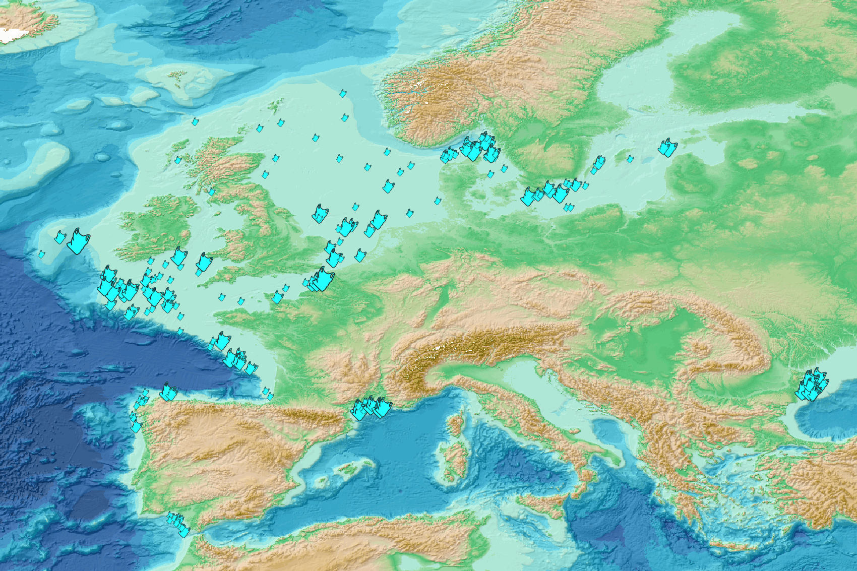
This visualization product displays plastic bags density per trawl. EMODnet Chemistry included the collection of marine litter in its 3rd phase. Since the beginning of 2018, data of seafloor litter collected by international fish-trawl surveys have been gathered and processed in the EMODnet Chemistry Marine Litter Database (MLDB). The harmonization of all the data has been the most challenging task considering the heterogeneity of the data sources, sampling protocols (OSPAR and MEDITS protocols) and reference lists used on a European scale. Moreover, within the same protocol, different gear types are deployed during fishing bottom trawl surveys. In cases where the wingspread and/or number of items were unknown, data could not be used because these fields are needed to calculate the density. Data collected before 2011 are affected by this filter. When the distance reported in the data was null, it was calculated from: - the ground speed and the haul duration using this formula: Distance (km) = Haul duration (h) * Ground speed (km/h); - the trawl coordinates if the ground speed and the haul duration were not filled in. The swept area is calculated from the wingspread (which depends on the fishing gear type) and the distance trawled: Swept area (km²) = Distance (km) * Wingspread (km) Densities have been calculated on each trawl and year using the following computation: Density of plastic bags (number of items per km²) = ∑Number of plastic bags related items / Swept area (km²) Percentiles 50, 75, 95 & 99 have been calculated taking into account data for all years. The list of selected items for this product is attached to this metadata. Information on data processing and calculation is detailed in the attached methodology document. Warning: the absence of data on the map doesn't necessarily mean that they don't exist, but that no information has been entered in the Marine Litter Database for this area.
-
This visualization product displays the number of Marine Strategy Framework Directive (MSFD) monitoring surveys and the associated temporal coverage per beach. EMODnet Chemistry included the collection of marine litter in its 3rd phase. Since the beginning of 2018, data of beach litter have been gathered and processed in the EMODnet Chemistry Marine Litter Database (MLDB). The harmonization of all the data has been the most challenging task considering the heterogeneity of the data sources, sampling protocols and reference lists used on a European scale. Preliminary processings were necessary to harmonize all the data: - Exclusion of OSPAR 1000 protocol: in order to follow the approach of OSPAR that it is not including these data anymore in the monitoring; - Selection of MSFD surveys only (exclusion of other monitoring, cleaning and research operations); - Exclusion of beaches without coordinates. More information is available in the attached documents. Warning: the absence of data on the map does not necessarily mean that they do not exist, but that no information has been entered in the Marine Litter Database for this area.
-

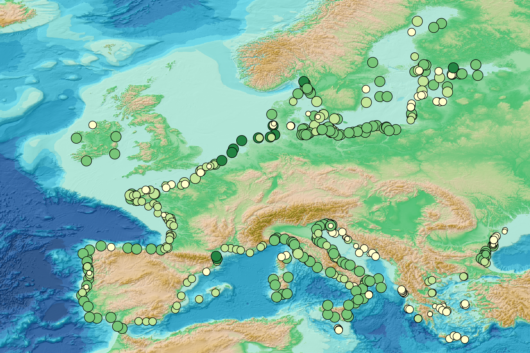
This visualization product displays the cigarette related items abundance of marine macro-litter (> 2.5cm) per beach per year from Marine Strategy Framework Directive (MSFD) monitoring surveys without UNEP-MARLIN data. EMODnet Chemistry included the collection of marine litter in its 3rd phase. Since the beginning of 2018, data of beach litter have been gathered and processed in the EMODnet Chemistry Marine Litter Database (MLDB). The harmonization of all the data has been the most challenging task considering the heterogeneity of the data sources, sampling protocols and reference lists used on a European scale. Preliminary processings were necessary to harmonize all the data: - Exclusion of OSPAR 1000 protocol: in order to follow the approach of OSPAR that it is not including these data anymore in the monitoring; - Selection of MSFD surveys only (exclusion of other monitoring, cleaning and research operations); - Exclusion of beaches without coordinates; - Selection of cigarette related items only. The list of selected items is attached to this metadata. This list was created using EU Marine Beach Litter Baselines, the European Threshold Value for Macro Litter on Coastlines and the Joint list of litter categories for marine macro-litter monitoring from JRC (these three documents are attached to this metadata); - Exclusion of surveys referring to the UNEP-MARLIN list: the UNEP-MARLIN protocol differs from the other types of monitoring in that cigarette butts are surveyed in a 10m square. To avoid comparing abundances from very different protocols, the choice has been made to distinguish in two maps the cigarette related items results associated with the UNEP-MARLIN list from the others; - Normalization of survey lengths to 100m & 1 survey / year: in some case, the survey length was not exactly 100m, so in order to be able to compare the abundance of litter from different beaches a normalization is applied using this formula: Number of cigarette related items of the survey (normalized by 100 m) = Number of cigarette related items of the survey x (100 / survey length) Then, this normalized number of cigarette related items is summed to obtain the total normalized number of cigarette related items for each survey. Finally, the median abundance of cigarette related items for each beach and year is calculated from these normalized abundances of cigarette related items per survey. Sometimes the survey length was null or equal to 0. Assuming that the MSFD protocol has been applied, the length has been set at 100m in these cases. Percentiles 50, 75, 95 & 99 have been calculated taking into account cigarette related items from MSFD monitoring data (excluding UNEP-MARLIN protocol) for all years. More information is available in the attached documents. Warning: the absence of data on the map does not necessarily mean that they do not exist, but that no information has been entered in the Marine Litter Database for this area.
-
Locations and associated attributes of circumpolar Muskox studies. Attributes include animal count, population estimate, estimate error and associated report citation.
-
Happywhale.com is a resource to help you know whales as individuals, and to benefit conservation science with rich data about individual whales. Original provider: Happywhale Dataset credits: Happywhale and contributors Supplemental information: Sightings and images were submitted to Happywhale by contributors. A portion of the Happywhale data were transferred to OBIS-SEAMAP upon the agreement between Happywhale and OBIS-SEAMAP. There may be duplicate records among Happywhale datasets and other OBIS-SEAMAP datasets. The precision of date/time vary per record. Some records have date accuracy up to year only. This dataset includes sightings and photos from the following 9 contributors in alphabetic order: Anna Astafurova; Barnaby; D Cavagnac; Hans Verdaat; Hondius; Jamie Coleman; Joel Moore; Philip Stone; Pippa Low