 Arctic SDI catalogue
RI_623
Type of resources
Available actions
Topics
Keywords
Contact for the resource
Provided by
Formats
Representation types
Update frequencies
status
Scale
-

Vertical seismic profiling (VSP) surveys done by the Geological Survey of Canada for research into downhole seismic imaging techniques for mineral exploration.
-
This data series represents the volumetric soil moisture (percent saturated soil) for the surface layer (<5 cm). The data is created daily and is averaged for the ISO standard week and month. The data is produced from passive microwave satellite data collected by the Soil Moisture and Ocean Salinity (SMOS) satellite and converted to soil moisture using version 6.20 of the SMOS soil moisture processor. The data are produced by the European Space Agency and obtained under a Category 1 proposal for Level 2 soil moisture data. The data are gridded to a resolution of 0.25 degrees. Data quality flags have been applied to remove areas where rainfall is present during the acquisition, where snow cover is detected and when Radio Frequency Interference (RFI) is above an acceptable threshold.
-
Monthly, seasonal and annual trends of mean hourly sea level and station pressure change (hectopascals) based on homogenized station data (AHCCD) are available. Trends are calculated using the Theil-Sen method using the station’s full period of available data. The availability of surface pressure trends will vary by station; if more than 5 consecutive years are missing data or more than 10% of the data within the time series is missing, a trend was not calculated.
-

Description: Seasonal mean total alkalinity from the British Columbia continental margin model (BCCM) were averaged over the 1981 to 2010 period to create seasonal mean climatology of the Canadian Pacific Exclusive Economic Zone. Methods: Total alkalinities at up to forty-six linearly interpolated vertical levels from surface to 2400 m and at the sea bottom are included. Spring months were defined as April to June, summer months were defined as July to September, fall months were defined as October to December, and winter months were defined as January to March. The data available here contain raster layers of seasonal total alkalinity climatology for the Canadian Pacific Exclusive Economic Zone at 3 km spatial resolution and 47 vertical levels. Uncertainties: Model results have been extensively evaluated against observations (e.g. altimetry, CTD and nutrient profiles, observed geostrophic currents), which showed the model can reproduce with reasonable accuracy the main oceanographic features of the region including salient features of the seasonal cycle and the vertical and cross-shore gradient of water properties. However, the model resolution is too coarse to allow for an adequate representation of inlets, nearshore areas, and the Strait of Georgia.
-

The Versatile Soil Moisture Budget (VSMB) is a soil water budget model that is continuous and deterministic in nature and was developed by AAFC. It is based on the premise that the water available for plant growth is gained by precipitation or irrigation, and lost through evapotranspiration and runoff as well as lateral and deep drainage. The daily net loss or gain is added or subtracted from the water already present in the rooting zone. Water is withdrawn simultaneously, but at different rates, from different soil depths, depending on the potential evapotranspiration, the stage of crop development, the water release characteristics of each soil layer and the available water.
-

A hydrogeological unit is defined as any soil or rock unit or zone that by virtue of its hydraulic properties has a distinct influence on the storage or movement of groundwater. It is considered the main dataset from the GGP point of view. Hydrogeological units are ranked into five levels (from largest to smallest): 1) hydrogeological region, 2) hydrogeological context, 3) aquifer system, 4) hydrostratigraphic unit, and 5) aquifer. Here are formal definitions for these different types of hydrogeologic units. - Hydrogeological region Hydrogeological regions are areas in which the properties of sub-surface water, or groundwater, are broadly similar in geology, climate and topography. There are 9 such regions identified in Canada (ref?). - Hydrogeological context Hydrogeological contexts are units of reporting, conceptually narrower than regions, and are additionally delineated by physiographic and hydrogeological aspects. - Aquifer system ""A heterogeneous body of intercalated permeable and poorly permeable material that functions regionally as a water-yielding hydraulic unit; it comprises two or more permeable beds [aquifers] separated at least locally by aquitards [confining units] that impede groundwater movement but do not greatly affect the regional hydraulic continuity of the system"" (Poland et al., 1972). - Hydrostratigraphic unit (HSU) ""Body of sediment and/or rock characterized by ground water flow that can be demonstrated to be distinct under both unstressed (natural) and stressed (pumping) conditions, and is distinguishable from flow in other HSUs"" (Noyes et al.) - Aquifer ""A formation, group of formations, or part of a formation that contains sufficient saturated permeable material to yield significant quantities of water to wells and springs"" (Lohman et al, 1972, p. 21). The rank attribute is used to specify the scope of the described unit. The general principle behind this specification is to allow the same data structure to apply to various types of hydrogeological units, from the local aquifer to the almost continental hydrogeological region. The dataset includes properties such as identification, physiography, geology, aquifer description and properties, water balance, groundwater use and risk. It features numerical values or a general description when no values are available. The description can also be used to add context to the numerical values. For each property, metadata identifying the source of the original data, links to similar data in GIN, and description of the processes, algorithms or methodology used to obtain these datasets will be available to complement the data. This dataset is designed to capture and represent a set of synthesized information pertaining to hydrogeological units through maps and succinct table reports. Some attributes (or properties) of the dataset are irrelevant depending of the rank of the unit. In general, this dataset is organised to include multiple properties associated with aquifers and larger hydrogeologic units. These properties are grouped into categories, which include identification, physiography, geology, aquifer description, water balance, groundwater use and risk. The numerical values associated with each of the properties can be used to create thematic maps; hence, the importance of using standardized units of measurement and definitions for these properties. When numerical values are not available, a general description may be supplied instead. The description can also be used to add context to the numerical values. Because this dataset is the cornerstone of the national view on groundwater, supplemental contextual information (metadata) must be part of the data. Thus, for each property, metadata identifying the source of the original data, links to similar data in GIN, and a description of the processes, algorithms or methodology used to obtain these datasets will be available to complement the data.
-

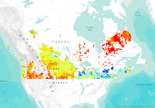
The Blended Index (BI) is a model which employs multiple potential indicators of drought and excess moisture, such as the Palmer drought index, rolling precipitation amounts and soil moisture, and combines them into a weighted, normalized value between 0 and 100. The inputs and weights used in this model are subject to change periodically as it is optimized to best represent extent, duration and severity of impactful weather conditions. The blended index is deployed as two variations; short term (st) focusing on 1 to 3 months, and long term (lt) focusing on 6 months to 5 years.
-

Growing Season Frost Free Period (-2 °C) is defined as the count of the number of days from the day after the last spring frost (-2 °C) to the day before the first fall frost (-2 °C). These values are calculated across Canada in 10x10 km cells.
-
This series includes maps of projected change in mean precipitation based on CMIP5 multi-model ensemble results for RCP2.6, RCP4.5 and RCP8.5, expressed as a percentage (%) of mean precipitation in the reference period. The median projected change across the ensemble of CMIP5 climate models is shown. Maps are provided for three time periods: 2016-2035, 2046-2065 and 2081-2100. For more maps on projected change, please visit the Canadian Climate Data and Scenarios (CCDS) site: https://climate-scenarios.canada.ca/?page=download-cmip5.
-

AIS NL Biofouling Species Fisheries and Oceans Canada's (DFO) National Marine Biofouling Monitoring Program conducts annual field surveys to monitor the introduction, establishment, spread, species richness, and relative abundance of native and some non-native species in Newfoundland and Labrador (NL) Region since 2006. Standardized monitoring protocols employed by DFO's NL, Maritimes, Gulf, and Quebec regions include biofouling collector plates deployed from May to October at georeferenced intertidal and shallow subtidal sites, including public docks, and public and private marinas and nautical clubs. Initially, (2006-2017), the collectors consisted of three 10 cm by 10 cm PVC plates deployed in a vertical array and spaced approximately 40 cm apart, with the shallowest plate suspended at least 1 m below the surface to sample subtidal and shallow intertidal species (McKenzie et al 2016a). Three replicate arrays were deployed at least 5 m apart per site. Since 2018, collector networks have been modified to improve statistical replication, including up to 10 individual collectors deployed per site at 1 m depth and at least 5 m apart (as above) from May to October. Since 2006, seven invasive biofouling organisms have been detected in Newfoundland and Labrador harbours, marinas and coastal areas. Should be cited as follows: DFO Newfoundland and Labrador Region Aquatic Invasive Species Marine Biofouling Monitoring Program. Published March 2024. Coastal and Freshwater Ecology, Northwest Atlantic Fisheries Centre, Fisheries and Oceans Canada, St. John’s, Newfoundland and Labrador. Reference: Tunicates Golden star tunicate (Botryllus schlosseri) 2006 The Golden star tunicate was the first invasive tunicate detected in NL waters. It was reported in Argentia by the US Navy around 1945. It was found in 2006 on wharf structures in Argentia, Placentia Bay during the first AIS survey (Callahan et al 2010). This colonial tunicate is recognized by it star shaped grouping of individuals within the colony. It is currently found in Placentia Bay, Fortune Bay, St. Mary’s Bay, Conception Bay and the west coast of NL. The data provided here indicates the detections of this AIS in coastal NL. From 2018-2022, the Coastal Environmental Baseline Program provided additional support to enhance sampling efforts in Placentia Bay.