 Arctic SDI catalogue
oceans
Type of resources
Available actions
Topics
Keywords
Contact for the resource
Provided by
Years
Formats
Representation types
Update frequencies
status
Scale
Resolution
-
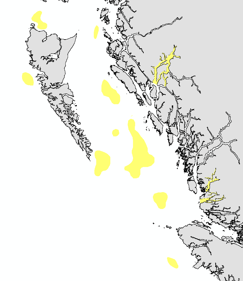
This layer details Important Areas (IAs) relevant to coral, sponge, and reef-building species in the Pacific North Coast Integrated Management Area (PNCIMA). This data was mapped to inform the selection of marine Ecologically and Biologically Significant Areas (EBSA). Experts have indicated that these areas are relevant based upon their high ranking in one or more of three criteria (Uniqueness, Aggregation, and Fitness Consequences). The distribution of IAs within ecoregions is used in the designation of EBSAs. Canada’s Oceans Act provides the legislative framework for an integrated ecosystem approach to management in Canadian oceans, particularly in areas considered ecologically or biologically significant. DFO has developed general guidance for the identification of ecologically or biologically significant areas. The criteria for defining such areas include uniqueness, aggregation, fitness consequences, resilience, and naturalness. This science advisory process identifies proposed EBSAs in Canadian Pacific marine waters, specifically in the Strait of Georgia (SOG), along the west coast of Vancouver Island (WCVI, southern shelf ecoregion), and in the Pacific North Coast Integrated Management Area (PNCIMA, northern shelf ecoregion). Initial assessment of IAs in PNCIMA was carried out in September 2004 to March 2005 with spatial data collection coordinated by Cathryn Clarke. Subsequent efforts in WCVI and SOG were conducted in 2009, and may have used different scientific advisors, temporal extents, data, and assessment methods. WCVI and SOG IA assessment in some cases revisits data collected for PNCIMA, but should be treated as a separate effort. Other datasets in this series detail IAs for birds, cetaceans, fish, geographic features, invertebrates, and other vertebrates. Though data collection is considered complete, the emergence of significant new data may merit revisiting of IAs on a case by case basis.
-
Moving 6-year analysis and visualization of Water body silicate in the North Sea. Four seasons (December-February, March-May, June-August, September-November). Data Sources: observational data from SeaDataNet/EMODnet Chemistry Data Network. Description of DIVA analysis: Geostatistical data analysis by DIVAnd (Data-Interpolating Variational Analysis) tool, version 2.7.9. results were subjected to the minfield option in DIVAnd to avoid negative/underestimated values in the interpolated results; error threshold masks L1 (0.3) and L2 (0.5) are included as well as the unmasked field. The depth dimension allows visualizing the gridded field at various depths.
-
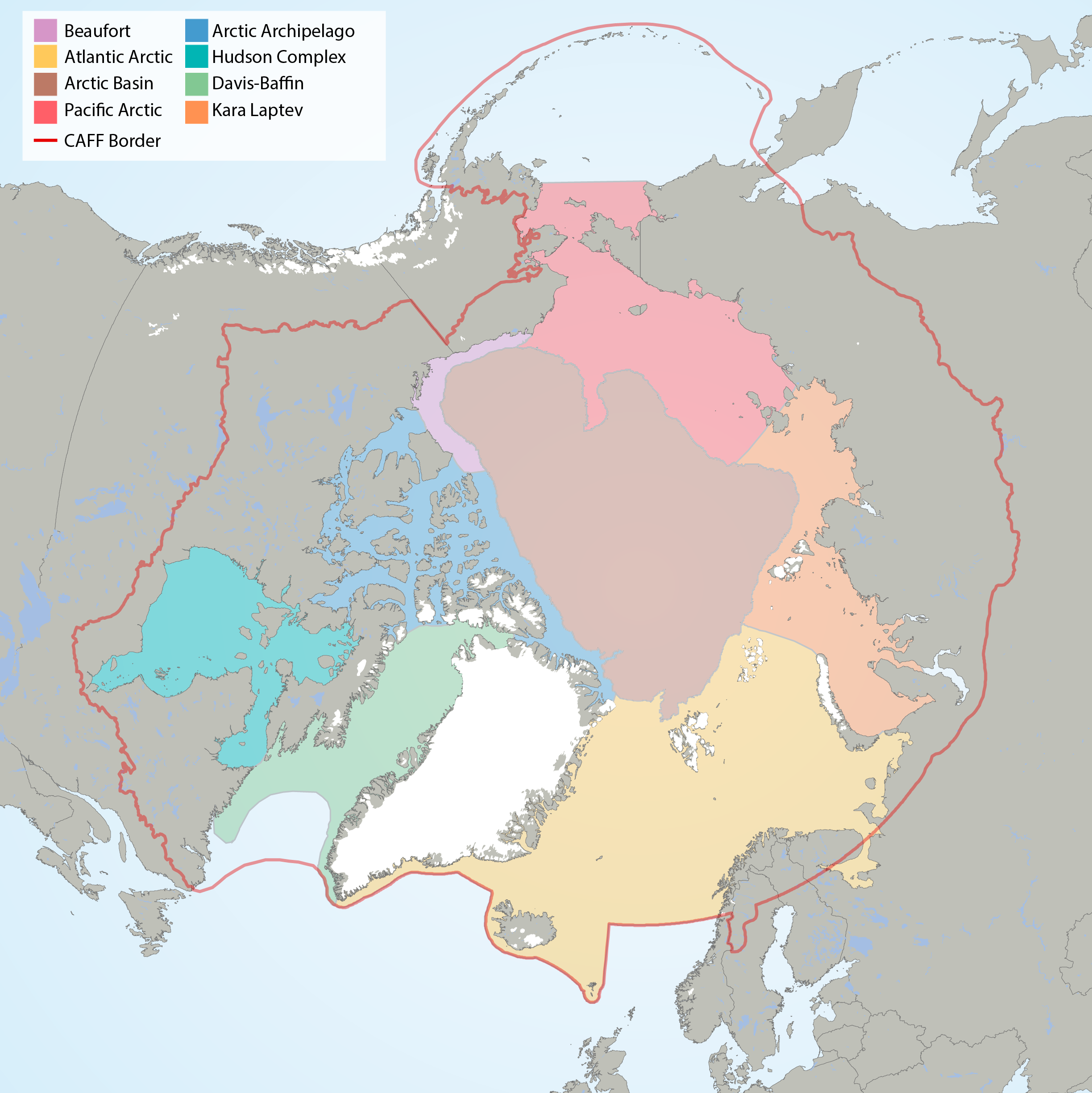
Arctic Marine Areas (AMAs) as defined in the CBMP Marine Plan. STATE OF THE ARCTIC MARINE BIODIVERSITY REPORT - <a href="https://arcticbiodiversity.is/marine" target="_blank">Chapter 1</a> - Page 15 - Figure 1.2
-
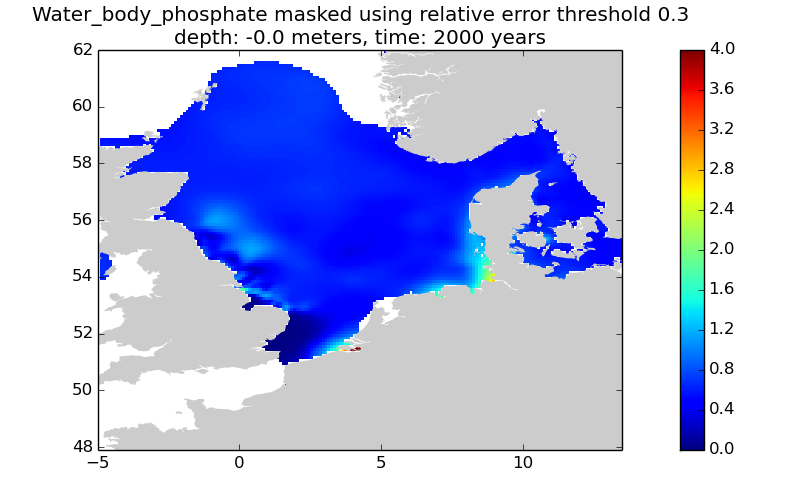
This gridded product visualizes 1960 - 2014 water body phosphate concentration (umol/l) in the North Sea domain, for each season (winter: December – February; spring: March – May; summer: June – August; autumn: September – November). It is produced as a Diva 4D analysis, version 4.6.9: a reference field of all seasonal data between 1960-2014 was used; results were logit transformed to avoid negative/underestimated values in the interpolated results; error threshold masks L1 (0.3) and L2 (0.5) are included as well as the unmasked field. Every step of the time dimension corresponds to a 10-year moving average for each season. The depth dimension allows visualizing the gridded field at various depths.
-
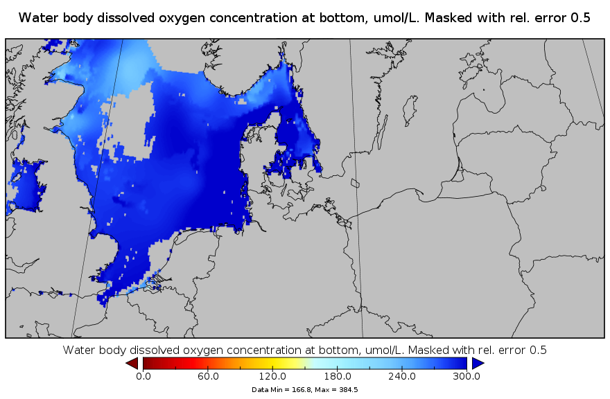
This gridded product visualizes 1960 - 2014 water body dissolved oxygen concentration (umol/l) in the North Sea domain, for each season (winter: December – February; spring: March – May; summer: June – August; autumn: September – November). It is produced as a Diva 4D analysis, version 4.6.11: a reference field of all seasonal data between 1960-2014 was used; results were logit transformed to avoid negative/underestimated values in the interpolated results; error threshold masks L1 (0.3) and L2 (0.5) are included as well as the unmasked field. Every step of the time dimension corresponds to a 10-year moving average for each season. The depth dimension allows visualizing the gridded field at various depths.
-
Long-term measurements of sea water properties collected by sensor buoy in Adventfjorden as part of the Svalbard Integrated Arctic Earth Observing System (SIOS).
-
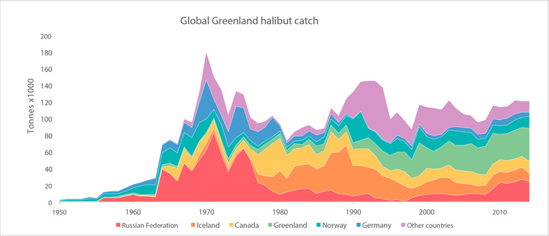
Global catches of Greenland halibut (FAO 2015). STATE OF THE ARCTIC MARINE BIODIVERSITY REPORT - <a href="https://arcticbiodiversity.is/findings/marine-fishes" target="_blank">Chapter 3</a> - Page 121 - Figure 3.4.8
-
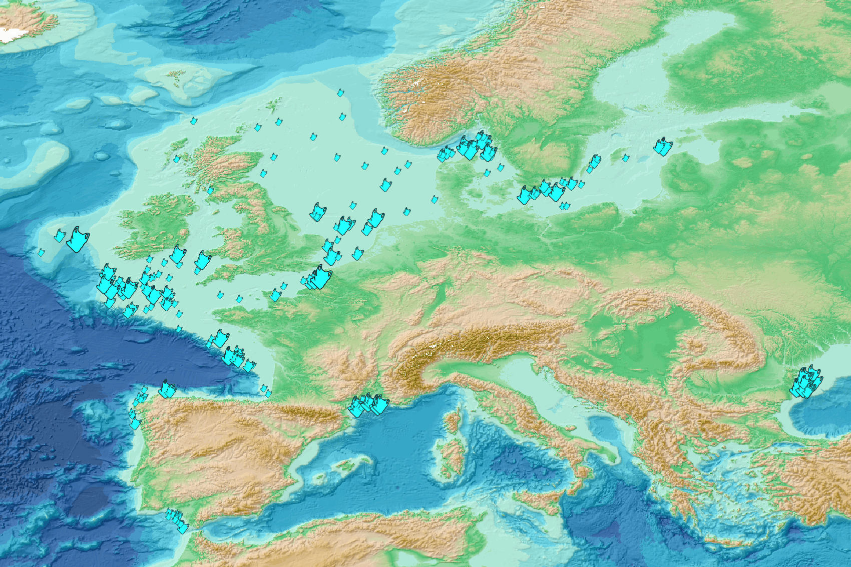
This visualization product displays plastic bags density per trawl. EMODnet Chemistry included the collection of marine litter in its 3rd phase. Since the beginning of 2018, data of seafloor litter collected by international fish-trawl surveys have been gathered and processed in the EMODnet Chemistry Marine Litter Database (MLDB). The harmonization of all the data has been the most challenging task considering the heterogeneity of the data sources, sampling protocols (OSPAR and MEDITS protocols) and reference lists used on a European scale. Moreover, within the same protocol, different gear types are deployed during fishing bottom trawl surveys. In cases where the wingspread and/or number of items were unknown, data could not be used because these fields are needed to calculate the density. Data collected before 2011 are affected by this filter. When the distance reported in the data was null, it was calculated from: - the ground speed and the haul duration using this formula: Distance (km) = Haul duration (h) * Ground speed (km/h); - the trawl coordinates if the ground speed and the haul duration were not filled in. The swept area is calculated from the wingspread (which depends on the fishing gear type) and the distance trawled: Swept area (km²) = Distance (km) * Wingspread (km) Densities have been calculated on each trawl and year using the following computation: Density of plastic bags (number of items per km²) = ∑Number of plastic bags related items / Swept area (km²) Percentiles 50, 75, 95 & 99 have been calculated taking into account data for all years. The list of selected items for this product is attached to this metadata. Information on data processing and calculation is detailed in the attached methodology document. Warning: the absence of data on the map doesn't necessarily mean that they don't exist, but that no information has been entered in the Marine Litter Database for this area.
-
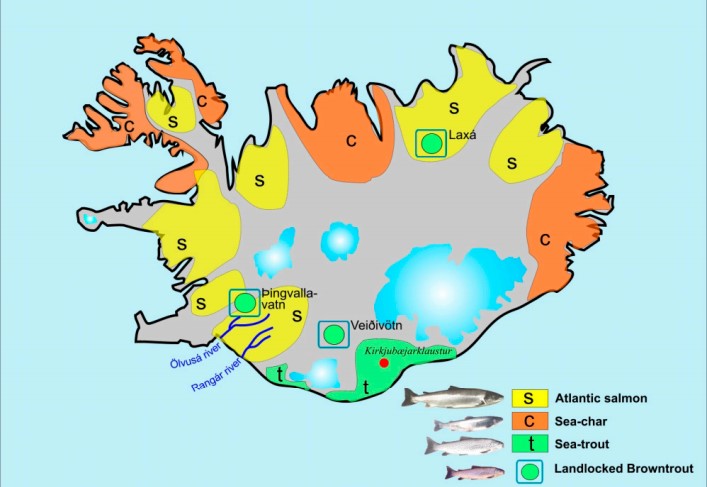
Vinsamlega hafið samband við Fiskistofu vegna nánari upplýsinga.
-
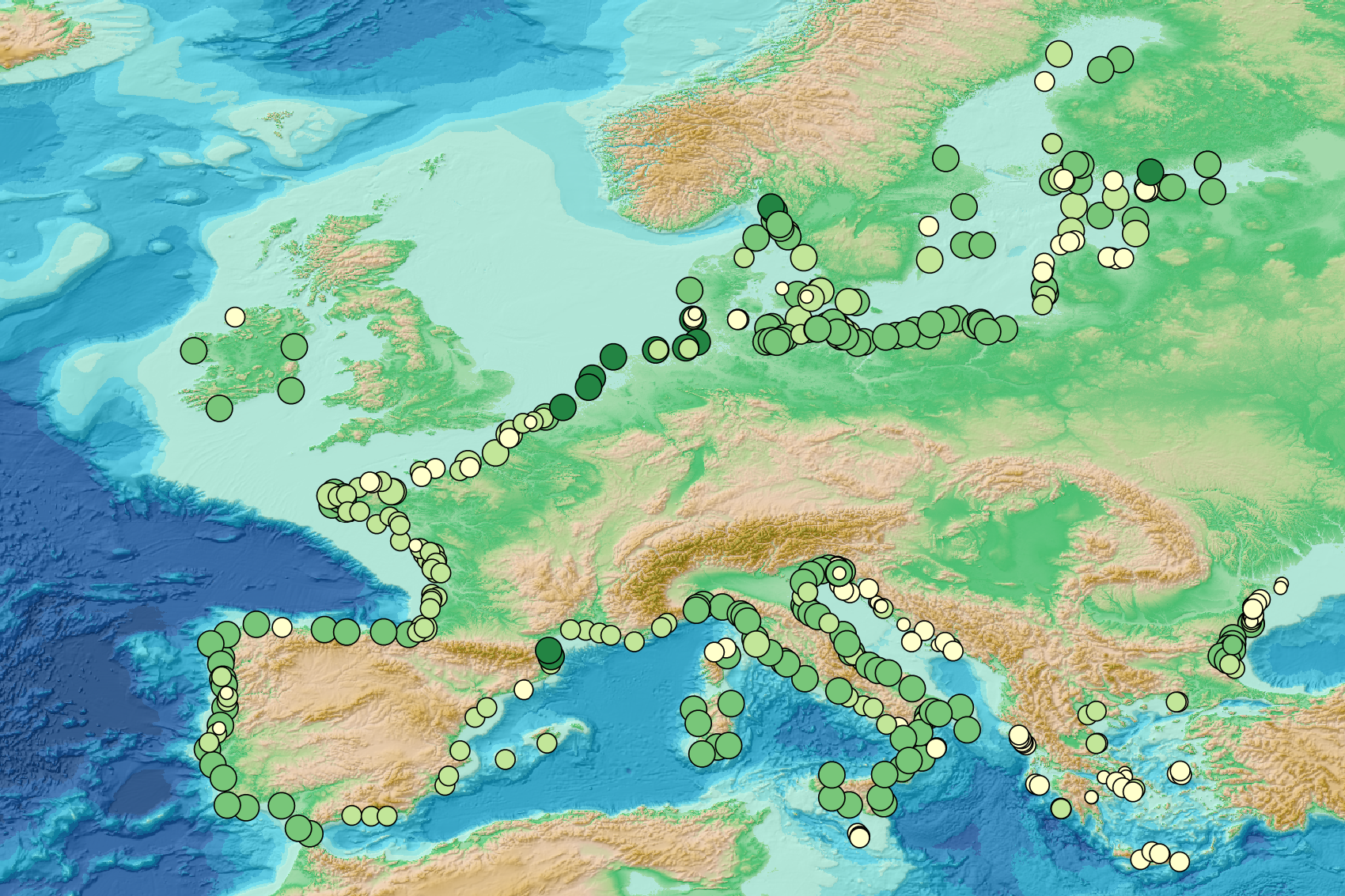
This visualization product displays the number of Marine Strategy Framework Directive (MSFD) monitoring surveys and the associated temporal coverage per beach. EMODnet Chemistry included the collection of marine litter in its 3rd phase. Since the beginning of 2018, data of beach litter have been gathered and processed in the EMODnet Chemistry Marine Litter Database (MLDB). The harmonization of all the data has been the most challenging task considering the heterogeneity of the data sources, sampling protocols and reference lists used on a European scale. Preliminary processings were necessary to harmonize all the data: - Exclusion of OSPAR 1000 protocol: in order to follow the approach of OSPAR that it is not including these data anymore in the monitoring; - Selection of MSFD surveys only (exclusion of other monitoring, cleaning and research operations); - Exclusion of beaches without coordinates. More information is available in the attached documents. Warning: the absence of data on the map does not necessarily mean that they do not exist, but that no information has been entered in the Marine Litter Database for this area.